
The Sun, Liquidity, and Financial Turning Points: The Regression Missed the Regime
A corrected Pattern Nexus analysis of solar cycles, liquidity, recessions, and financial tops from January 1987 through July 2026. The first monthly regression rejected a short-horizon trading signal. The properly specified regime test found that all four U.S. recession onsets in the sample occurred within twelve months of an official solar maximum or minimum, recession months were sharply concentrated around those extrema, and M2 growth was faster on official solar rising legs.
The regression did not kill the thesis. It exposed the correct horizon.
I have said it in plain language: as the sun rises in power, so does liquidity. The original test translated that into short monthly solar changes and asked whether those changes improved near-term financial forecasts. That test produced a clean failure. None of the ten core short-horizon model tests met the corrected decision rule.
But that was not the actual claim. The Pattern Nexus claim was always a regime claim: solar ascent, liquidity expansion, financial excess, a turning zone, contraction, and reset. Once I tested official solar legs and official solar turning points instead of monthly wiggles, the result changed.
- Four out of four U.S. recession onsets from January 1987 through July 2026 occurred within ±12 months of an official solar maximum or minimum.
- The exact circular timing test produced p = 0.048. Correcting for the choice among several reasonable window widths moved that to p = 0.067.
- Removing the plainly exogenous March 2020 onset left three out of three recession starts inside the window, with p = 0.072.
- Recession months represented 18.3% of months near solar extrema and only 1.3% of months outside those windows. The duration-preserving circular test produced p = 0.013.
- U.S. M2 growth averaged 6.80% on official solar rising legs and 4.72% on falling legs, a +2.08 percentage-point difference. The directional timing test produced p = 0.058.
That is not proof that the sun causes recessions. It is not a mechanical market clock. It is not permission to ignore credit, rates, collateral, fiscal policy, technology, war, or policy error. It is evidence that solar phase belongs inside the Pattern Nexus regime map as a warning variable—especially when liquidity, credit, rates, and collateral are already moving in the same direction.
Yes, the correlation is visible. It was hiding in the turning points.
The honest answer is yes. I can see the correlation now. More importantly, I can specify what kind of correlation it is.
It is not a stable month-to-month relationship in which a one-unit increase in sunspots produces a fixed increase in M2, the NASDAQ, housing, or the Pattern Nexus liquidity composite a few months later. That linear version does not survive the data. The relationship is nonlinear and regime-based. It appears most clearly at the boundaries: the places where an expansion becomes exhaustion, where a contraction becomes reset, and where the financial system is already fragile enough for a trigger to matter.
That distinction matters because a regime tool can be useful even when it cannot forecast the next monthly return. Credit cycles, demographic cycles, capital-expenditure cycles, commodity cycles, and political cycles work the same way. The broad phase changes the probability distribution. It does not dictate every observation.
“As the sun rises in power, so does liquidity” is a regime hypothesis.
The claim is not that bankers check the sunspot count before extending credit. It is not that the Federal Reserve mechanically follows the sun. It is not that a solar maximum produces a stock-market peak on the same date. That would be easy to reject because the world does not work with that kind of precision.
The actual claim is that the approximately eleven-year solar cycle may sit above several slower systems that shape the background conditions for production, confidence, surplus, credit formation, and financial risk. In my own framework, the proposed historical chain is:
That chain is easiest to understand in agrarian history. A civilization with better harvests produces more surplus. More surplus supports trade, taxation, lending, construction, state capacity, and asset accumulation. A civilization hit by repeated harvest stress experiences the opposite: tighter food balances, political stress, impaired debt service, and less financial flexibility.
The modern financial system is not an agrarian village enlarged. Central banks can create reserves. Governments can run deficits. Private banks can expand balance sheets. Energy systems, storage, insurance, global trade, fertilizer, and technology can buffer local climate shocks. So the historical mechanism cannot simply be pasted onto M2.
But modern finance is still built on real surplus, collateral, income, confidence, and the willingness to extend claims on the future. The proposed mechanism is therefore a background envelope, not a direct pipe. If the solar cycle matters, it should appear as a slow change in regime probabilities—not as a clean daily or monthly beta.
That is what this study tests.
First fix the official solar dates.
There is a trap in cycle research: the chart shape is broad, memory compresses several years into one phase, and we start calling an entire basin a “minimum” or an entire plateau a “maximum.” That may be acceptable in conversation. It is not acceptable in a regression.
WDC–SILSO defines the official cycle extrema from the 13-month smoothed monthly sunspot number. For the period in this study, the dates are precise: Cycle 22 reached maximum in November 1989; Cycle 23 began at the August 1996 minimum and reached maximum in November 2001; Cycle 24 began at the December 2008 minimum and reached maximum in April 2014; Cycle 25 began at the December 2019 minimum and reached maximum in October 2024.[1][2]
| Solar event | Official month | Smoothed sunspot number | Financial interpretation used here |
|---|---|---|---|
| Cycle 22 minimum | September 1986 | 13.5 | Starting point of the rising leg entering the sample. |
| Cycle 22 maximum | November 1989 | 212.5 | Late-cycle turning zone near the 1990 recession. |
| Cycle 23 minimum | August 1996 | 11.2 | Reset and start of the 1996–2001 rising leg. |
| Cycle 23 maximum | November 2001 | 180.3 | Turning zone around the technology bust and 2001 recession. |
| Cycle 24 minimum | December 2008 | 2.2 | Terminal crisis/reset zone after housing and credit broke. |
| Cycle 24 maximum | April 2014 | 116.4 | Weak-cycle maximum; no U.S. recession onset nearby. |
| Cycle 25 minimum | December 2019 | 1.8 | Reset zone immediately before the exogenous 2020 recession. |
| Cycle 25 maximum | October 2024 | 160.9 | Current turning point; the system is now on the declining leg. |
This corrects two common descriptions. The 1997–2001 period was not a solar minimum; it was the rising leg from the August 1996 minimum into the November 2001 maximum. And 2006 was not the official solar maximum; it was the housing top on the declining leg from the 2001 maximum toward the December 2008 minimum.
The larger financial intuition survives those corrections. In fact, it becomes more coherent. The technology cycle broke around a solar maximum. The housing and credit system broke while descending into a solar minimum. The relevant object is the turning architecture, not a mislabeled year.
I asked a monthly model to answer a multi-year question.
The first workbook treated solar variables the way a conventional factor model would. It took monthly changes, slopes, and phase measures, added them to financial models, and asked whether the solar term improved short-horizon forecasts after normal controls.
The answer was no. The ten core models did not provide a robust, corrected short-horizon solar signal. Longer lead scans also failed to produce a stable forecasting relationship after the search across lags was penalized. Those results are real. I am not deleting them because the corrected test is more interesting.
But the headline I initially drew from them—effectively “zero for ten, no solar-financial relationship”—was too broad. The test rejected one version of the claim: a linear, incremental, monthly forecasting factor. It did not test whether recessions and financial turning points cluster around official solar extrema, and it did not test whether broad money behaves differently across full rising and falling legs.
What the first test asked
Does a monthly solar variable add near-term predictive power after standard controls?
What my thesis actually asked
Do liquidity and financial stress organize differently across multi-year solar phases and turning zones?
What still failed
No stable monthly trading beta and no corrected 0–72 month lead that survived the full search.
What became visible
Recession timing near extrema, recession-state concentration, and faster average M2 growth on rising legs.
Turn the story into an event study and a phase test.
The corrected analysis uses January 1987 through July 2026 as the common monthly calendar. Solar activity comes from the WDC–SILSO monthly and 13-month smoothed sunspot series. Official extrema come from the SILSO minimum/maximum chronology. U.S. recession months come from FRED’s monthly NBER-based recession indicator. M2 is the Federal Reserve’s seasonally adjusted monthly M2 series distributed through FRED.[1][3][4][5]
The analysis asks four separate questions:
- Turning-point timing: Is the first month of each U.S. recession unusually close to an official solar maximum or minimum?
- Recession-state concentration: Are recession months more common inside the turning-point windows than outside them?
- Phase direction: Is M2 growth faster on official minimum-to-maximum rising legs than on maximum-to-minimum falling legs?
- Forecasting robustness: Do solar level or slope variables produce stable low-frequency leads after the full 0–72 month search is corrected?
For turning-point timing, I define a window of ±12 months around each official extremum. The observed four-recession pattern is then shifted around the full calendar one month at a time. This preserves the spacing between recessions while breaking the alignment with the solar dates. The exact p-value is the share of circular shifts that place at least as many recession starts inside the windows as the observed alignment.
The ±12-month window was not the only width inspected. I also tested ±6, ±18, ±24, ±30, and ±36 months. Because choosing the best-looking width after seeing the data can manufacture significance, the workbook includes a max-over-window correction. The raw ±12-month timing result is p = 0.048. After the window search is penalized, it is p = 0.067.
For recession-state concentration, I shift the full monthly recession vector instead of only the four start months. This preserves recession duration and clustering. For the M2 phase test, I shift the full rising/falling phase pattern against M2 growth, preserving the long blocks that define a cycle regime.
These are small-sample exact timing tests. They do not turn three and a half solar cycles into forty years of independent evidence. The true low-frequency degrees of freedom are measured in cycles, not monthly rows. That limitation stays visible throughout the article.
The chart tells the story the first regression could not.
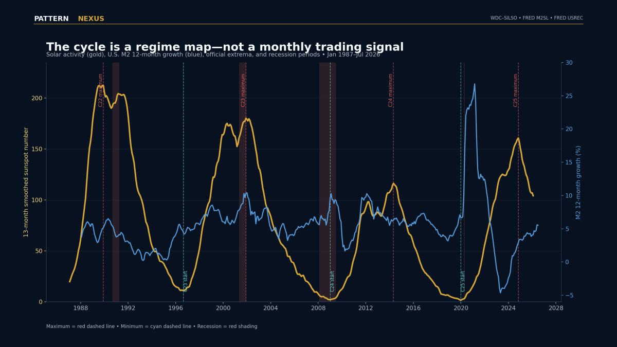
Look at the chart as a sequence of regimes, not as two lines that must move together every month.
The late-1980s solar rise reaches the powerful November 1989 maximum. The 1990 recession begins nine months later. The system then moves down toward the August 1996 solar minimum. From that minimum, the next solar rising leg overlaps the technology, telecom, globalization, and credit expansion of the late 1990s. The April 2001 recession begins seven months before the official November 2001 maximum.
The 2001–2008 declining solar leg contains the housing peak, the leverage build, the 2007 market top, the credit break, and the January 2008 recession onset. That recession begins eleven months before the December 2008 solar minimum. The minimum does not cause the housing bubble. It marks the terminal zone of a declining phase in which the financial system’s accumulated leverage finally breaks.
The 2008 minimum then gives way to a new rising solar leg and the post-crisis monetary expansion. The 2019 minimum sits immediately before the pandemic shock and the largest synchronized fiscal-monetary expansion in the modern sample. Cycle 25 rises into the official October 2024 maximum. We are now on the declining leg from that maximum.
The blue M2 line is not a copy of the gold solar line. It should not be. M2 responds to policy, regulation, fiscal transfers, banking behavior, and crisis intervention. The claim supported by the data is narrower: M2 growth is faster on average during official rising legs, while recession stress is unusually concentrated around the extrema.
The sequence matters more than any one date.
1987–1996: the Cycle 22 maximum and the 1990 recession
The sample begins on the rising leg of Cycle 22. Solar activity accelerates into the November 1989 maximum, the strongest official maximum inside this study. The objective NASDAQ pre-recession peak occurs in September 1989, two months before the solar maximum. The national housing index reaches its pre-recession peak in July 1990, eight months after the maximum. The recession begins in August 1990, nine months after the maximum.
This is the cleanest maximum-side alignment in the sample. The market peak, housing peak, solar maximum, and recession onset all occupy the same broad turning zone. But even here, the dates do not collapse into one month. Markets price the transition before the recession indicator turns on. Housing is slower. The recession begins after the extremum.
The falling leg from the 1989 maximum to the August 1996 minimum averages only 2.88% M2 growth in the leg-level table. That is the weakest complete falling-leg M2 average in the sample. It overlaps recession, banking stress, commercial-real-estate damage, and the long repair that follows.
1996–2001: the solar rise, the technology boom, and the 2001 break
August 1996 is the official solar minimum. From there, solar activity rises toward the November 2001 maximum. The financial system simultaneously enters the most visible speculative technology expansion of the period: cheapening communications, internet adoption, capital-market enthusiasm, venture funding, equipment investment, and a historic rise in the NASDAQ.
It would be easy to overstate this. The sun did not invent the internet. Monetary policy, productivity expectations, tax rules, telecommunications deregulation, venture capital, and investor psychology did the direct work. The solar phase is a candidate background regime, not a substitute for those explanations.
The objective NASDAQ peak occurs in February 2000, twenty-one months before the official solar maximum. Housing reaches its pre-recession peak in April 2001. The recession also begins in April 2001, seven months before the solar maximum. This is why the correct window must be broad enough to represent a turning zone but narrow enough to be falsifiable.
The official 1996–2001 rising leg averages 6.68% M2 growth. The recession begins while the solar cycle is late-rising and near maximum. In the Pattern Nexus interpretation, this is an exhaustion-side event: the expansion builds on the rising leg, the speculative market tops before the official maximum, and the economic contraction arrives inside the maximum turning zone.
2001–2008: housing tops on the way down, not at a 2006 solar maximum
This is the chronology that matters most because it can be mislabeled in casual discussion. The official solar maximum was November 2001. There was no official 2006 solar maximum. The housing peak in July 2006 occurred fifty-six months after the 2001 maximum and twenty-nine months before the December 2008 minimum.
That does not erase the relationship. It changes the relationship. The housing bubble peaks during the descending solar leg. The NASDAQ makes its objective pre-recession peak in October 2007, fourteen months before the solar minimum. The recession begins in January 2008, eleven months before the minimum. The crisis reaches maximum intensity as the solar cycle reaches its trough.
This is a contraction-side alignment. It is different from 1990 and 2001, which cluster around maxima. A solar maximum can align with late-cycle exhaustion. A solar minimum can align with terminal liquidation and reset. Both are extrema, but they represent opposite boundaries of the phase map.
The 2001–2008 falling leg still averages 6.06% M2 growth, which is not low. That matters. Broad money can continue expanding while credit quality deteriorates and leverage becomes unstable. M2 alone does not measure underwriting standards, off-balance-sheet leverage, mortgage fraud, wholesale funding, or collateral fragility. The mechanism is not “falling sun equals falling money every year.” It is “falling phase changes the regime, while the financial system can keep extending itself until the collateral stack breaks.”
2008–2014: the minimum is a basin, then the rebuilding leg begins
December 2008 is the official minimum. The broader 2008–2009 period is visually a solar basin, which is why people often describe 2008–2012 as “the minimum.” Officially, however, 2009–2012 is the rising leg of Cycle 24. The difference is not cosmetic. The minimum is the turning point; the years after it are the reconstruction phase.
That reconstruction coincides with emergency monetary policy, quantitative easing, bank recapitalization, fiscal support, mortgage intervention, and a long rebuilding of financial balance sheets. M2 growth averages 6.67% from the December 2008 minimum to the April 2014 maximum. Gold performs strongly through the crisis and sovereign-risk aftermath. Equities recover. Housing lags because foreclosures, impaired borrowers, negative equity, and damaged credit transmission continue to dominate the asset even after central-bank liquidity expands.
This episode is one of the best demonstrations of the difference between liquidity regime and asset timing. A new rising leg can support the system without making every asset turn on the same date. Housing has a slower and more damaged transmission mechanism than publicly traded equities or gold.
2014–2019: a declining solar leg without a U.S. recession
Cycle 24 reaches its relatively weak maximum in April 2014. The next official minimum does not arrive until December 2019. No U.S. recession begins within twelve months of the 2014 maximum. That is important because the framework must show its false alarms and empty windows.
Not every solar extremum produces a recession. The fact that all four recessions occur near extrema is not the same as saying every extremum causes recession. In conditional-probability language, the study finds a strong in-sample value for “recession start given the calendar is near an extremum,” but it does not produce a perfect value for “recession given any extremum.”
The 2014–2019 falling leg averages 5.52% M2 growth. Equities and housing continue to advance through much of the period, supported by low rates, earnings growth, global balance-sheet conditions, mortgage lock-in effects beginning to form, and a financial system far less impaired than it was in 2008. Solar phase is not sufficient. Financial vulnerability still has to exist.
2019–2024: minimum, pandemic shock, liquidity eruption, and a new maximum
Cycle 25 begins at the December 2019 minimum. The objective NASDAQ pre-recession peak occurs in January 2020, one month after the minimum. The recession begins in March 2020, three months after the minimum. Housing’s pre-recession peak is also March 2020 in the mechanical lookback rule.
The initiating shock was a pandemic. It was exogenous to any plausible solar-financial mechanism. That is why the workbook repeats the test without 2020. Removing it leaves the other three recession starts inside the ±12-month window, but the exact p-value weakens to 0.072 because the already-small event count becomes smaller.
Then the rising leg overlaps the most aggressive M2 expansion in the sample. The official December 2019–October 2024 rising leg averages 7.85% M2 growth, the strongest complete rising-leg average in the study. That number includes extraordinary fiscal transfers, central-bank asset purchases, emergency lending, deposit creation, and the later normalization. The solar phase did not create those policies. It identifies the regime in which the largest liquidity event occurred.
Cycle 25 reaches its official maximum in October 2024. The financial system has since moved onto the declining solar leg. That does not mean an immediate recession was due in October 2024 or is mechanically due now. It means the regime map has moved from ascent toward descent, and confirmation variables deserve more weight.
Four recessions. Four solar turning zones.
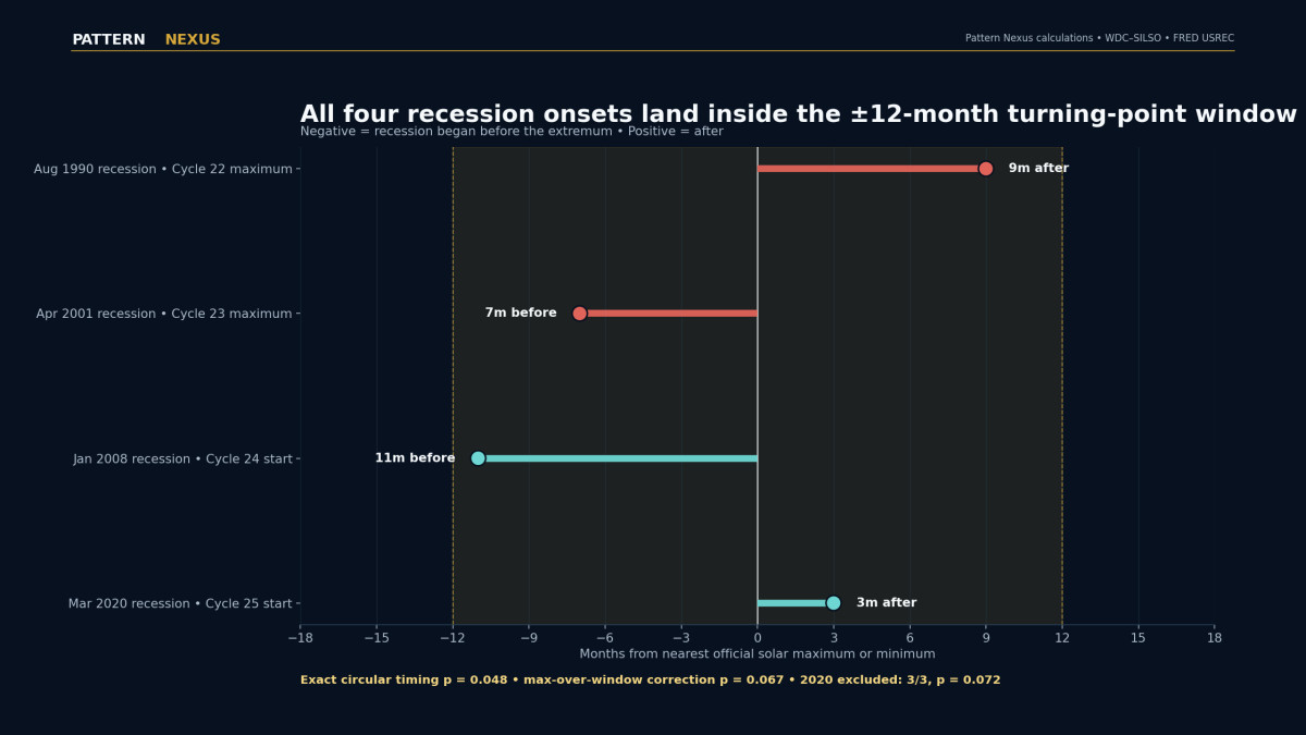
| Recession onset | Nearest extremum | Type | Signed distance | Inside ±12 months? |
|---|---|---|---|---|
| August 1990 | November 1989 | Maximum | +9 months | Yes |
| April 2001 | November 2001 | Maximum | −7 months | Yes |
| January 2008 | December 2008 | Minimum | −11 months | Yes |
| March 2020 | December 2019 | Minimum | +3 months | Yes |
The ±12-month windows cover 175 of the 475 months in the study, or 36.8% of the calendar. If recession starts were unrelated to the solar dates, the expected number of starts inside the windows would be about 1.47. The observed number is four.
Under the exact circular timing test, only 4.84% of the possible shifts match or exceed that alignment. That produces p = 0.048. When the analysis penalizes the fact that six window widths were inspected, the corrected p-value becomes 0.067.
I am not going to pretend that 0.067 is the same thing as a clean out-of-sample discovery. It is not. It is statistically suggestive in a tiny cycle sample. The result earns a place in the model and a demand for more testing. It does not earn a claim of physical causation.
Recession is not just starting near the extrema. It is concentrated there.
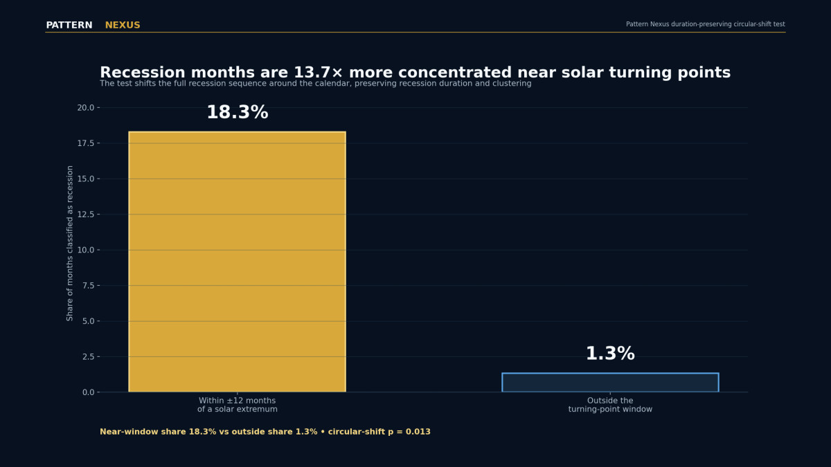
This is the strongest statistical result in the corrected workbook. Instead of reducing each recession to one start month, the test uses the entire monthly recession state. It then shifts that full pattern around the calendar, preserving how long each recession lasted.
The observed difference is large: 18.3% of months inside the turning-point windows are recession months, compared with 1.3% outside. That is not a claim that 18.3% of every future turning window will be recession. It is the sample result from these cycles.
The duration-preserving circular test produces p = 0.013. In other words, the recession state is more concentrated around the official solar extrema than almost all timing shifts that preserve the same recession lengths.
There is still an important caveat. The long 2007–2009 recession sits around the December 2008 solar minimum and contributes many recession months to the near-window count. The test preserves that duration under the null, which is the correct way to avoid treating each recession month as independent. But the economic interpretation still depends heavily on one historic crisis. More cycles are the only real cure for that limitation.
Broad money grew faster while solar power was rising.
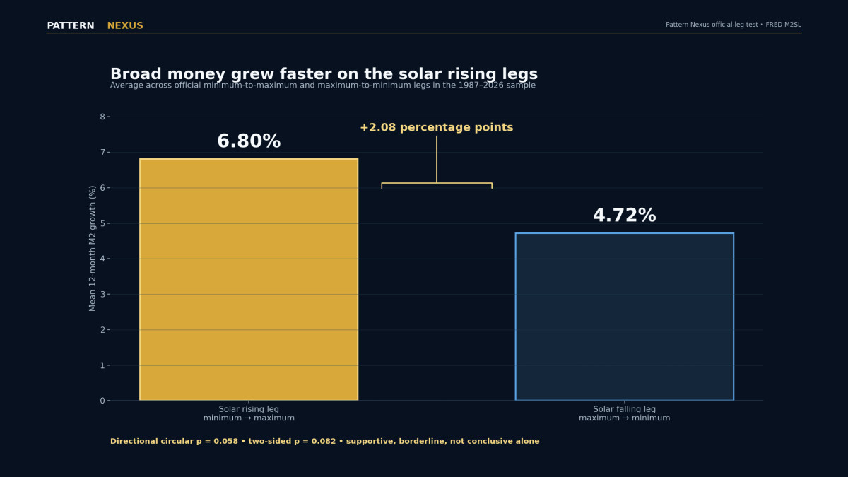
This is the result closest to my original wording. Across all usable months, M2 growth averages 2.08 percentage points faster on rising solar legs than on falling legs.
The directional p-value is 0.058. That is borderline evidence in the predicted direction. The two-sided p-value is 0.082. Neither number supports a claim of certainty. Both are strong enough that dismissing the difference as invisible would also be wrong.
| Official leg | Phase | Months in sample | Mean M2 12-month growth | What it shows |
|---|---|---|---|---|
| Cycle 22 start → Nov. 1989 max | Rising | 35 | 4.74% | Strong solar rise, but M2 growth was not unusually high. |
| Nov. 1989 max → Aug. 1996 min | Falling | 82 | 2.88% | Weakest complete falling-leg M2 average. |
| Aug. 1996 min → Nov. 2001 max | Rising | 64 | 6.68% | Technology and credit expansion on the rising leg. |
| Nov. 2001 max → Dec. 2008 min | Falling | 86 | 6.06% | Money growth remained high while private credit quality deteriorated. |
| Dec. 2008 min → Apr. 2014 max | Rising | 65 | 6.67% | Post-crisis policy expansion and balance-sheet repair. |
| Apr. 2014 max → Dec. 2019 min | Falling | 69 | 5.52% | Declining phase without a U.S. recession onset. |
| Dec. 2019 min → Oct. 2024 max | Rising | 59 | 7.85% | Largest rising-leg M2 average, dominated by the pandemic response. |
The leg table prevents a seductive average from becoming a false law. The 2001–2008 falling leg had faster M2 growth than the early Cycle 22 rising leg. The relationship is probabilistic and conditional. Policy can overwhelm it. Private credit can expand even while the broader regime becomes more fragile. M2 is one liquidity channel, not the entire financial system.
The financial peaks cluster around the extrema, but they do not share one clock.
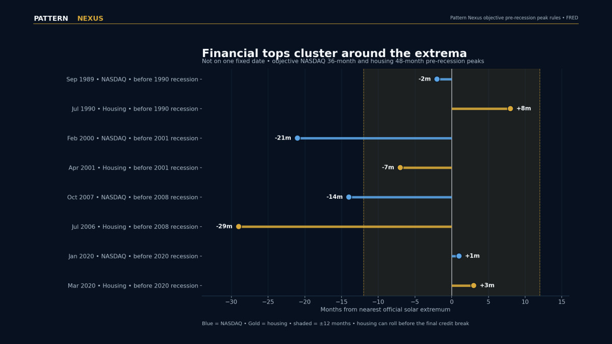
The market-top test is intentionally mechanical. For each recession, I select the highest NASDAQ level in the prior thirty-six months and the highest national home-price level in the prior forty-eight months. That keeps the narrative from moving the peak date after seeing the solar chart.
The results show both the appeal and the limit of the thesis. The 1989 NASDAQ peak is two months before the Cycle 22 maximum. The 1990 housing peak is eight months after it. The 2001 housing peak is seven months before the Cycle 23 maximum. The 2020 market and housing peaks are within three months of the Cycle 25 minimum.
But the February 2000 NASDAQ peak is twenty-one months before the 2001 maximum. The July 2006 housing peak is twenty-nine months before the 2008 minimum. The October 2007 NASDAQ peak is fourteen months before the minimum. Those are broad-cycle alignments, not precise ±12-month hits.
That is exactly what different transmission speeds should produce. Public equities can reprice rapidly when earnings expectations, discount rates, or risk appetite change. Housing turns slowly because listings, appraisals, mortgage approvals, construction, and distressed inventory operate with long lags. Credit can continue expanding after collateral quality has begun to deteriorate. A single date would be suspiciously neat.
LCI4 points in the expected direction, but the sample is not strong enough.
The article cannot stop at M2 because my own liquidity framework is broader. Pattern Nexus LCI4 combines four traditional liquidity reservoirs: the Federal Reserve balance sheet, inverted Treasury General Account, inverted overnight reverse-repo balance, and M2. The point is to measure a financing environment, not to pretend one monetary series is “liquidity.”[6][7]
The exact published LCI4 series available for this test begins in February 2003 and runs through June 2026. Its 12-month change averages 0.193 standard-deviation units on solar rising legs and 0.026 on falling legs, a difference of +0.167 in the predicted direction.
That difference is not statistically robust. The directional circular p-value is approximately 0.201, and the two-sided p-value is approximately 0.335. The series only covers a little more than two solar cycles and includes extraordinary changes in reserve policy, Treasury cash management, the reverse-repo facility, and pandemic-era money creation.
This is a reason to keep the variable, not a reason to market it as proven. The M2 phase result is stronger than the LCI4 result in this sample. The recession-turning-point result is stronger than both.
The model hierarchy therefore matters:
- Primary finding: recession timing and recession-state concentration around solar extrema.
- Secondary finding: faster average M2 growth on rising solar legs.
- Exploratory finding: LCI4 changes are directionally stronger on rising legs but not statistically reliable.
- Rejected claim: a stable short-horizon solar coefficient that works as a monthly trading signal.
The data does not give me a clean lead time.
I also tested low-frequency leads from zero through seventy-two months. The predictors included the solar level and a multi-year solar slope. The targets included M2 trend growth, gold, NASDAQ, housing, the Pattern Nexus LCI4 trend, and a descriptive financial-cycle composite.
There were twelve predictor-target scans. After each scan was corrected for searching every lead and the resulting tests were corrected across the family, zero of twelve survived a Benjamini–Hochberg false-discovery threshold of q < 0.05. The best corrected q-value was approximately 0.571.
That result blocks the strongest forecasting claim. I cannot use this sample to say that solar activity leads M2 or markets by one fixed number of months. The data supports a phase classifier and a turning-point warning zone. It does not support a universal lag.
This is not a minor distinction. A model that says “solar maximum means the market peaks exactly X months later” invites false precision and backtest selection. A model that says “the system has entered a boundary regime; now require confirmation from liquidity, credit, rates, and collateral” is slower, less dramatic, and more consistent with the evidence.
Why four out of four is meaningful—and why it is still not enough.
A result can look dramatic and still be statistically empty if the window is so wide that almost every month qualifies. That is the first thing I wanted to prevent.
At ±12 months around the official extrema, the windows cover 36.8% of the January 1987–July 2026 calendar. That is a large share, but it is nowhere near the whole calendar. With four recession onsets and no relationship, the simple calendar expectation is about 1.47 recession starts inside those windows. The observed count is four.
The circular test asks a stricter question. Keep the observed distance between the four recession starts exactly as it occurred. Move the complete four-event pattern ahead by one month. Count how many shifted starts land inside the fixed solar windows. Repeat that operation for every possible shift around the 475-month calendar. The p-value is the fraction of shifts that do at least as well as the real dates.
That matters because recessions are not independent lottery balls. Their spacing is part of the macro structure. A circular shift preserves that spacing. It destroys only the alignment with the solar chronology.
| Window around each extremum | Starts inside | Calendar covered | Starts expected if unrelated | Exact circular p |
|---|---|---|---|---|
| ±6 months | 1 of 4 | 19.2% | 0.77 | 0.524 |
| ±12 months | 4 of 4 | 36.8% | 1.47 | 0.048 |
| ±18 months | 4 of 4 | 54.5% | 2.18 | 0.152 |
| ±24 months | 4 of 4 | 71.6% | 2.86 | 0.352 |
| ±30 months | 4 of 4 | 87.4% | 3.49 | 0.608 |
| ±36 months | 4 of 4 | 95.8% | 3.83 | 0.848 |
This table is the reason the ±12-month result is interesting. A ±6-month window is too narrow for three of the four recession starts. At ±18 months and beyond, all four starts still qualify, but the window covers so much of the calendar that the result becomes progressively less surprising. By ±36 months, almost the entire sample is “near” an extremum and the test has nearly no discriminatory power.
The ±12-month window is the point at which the observed count jumps from one to four while the calendar coverage remains below forty percent. That makes it the strongest observed window. But selecting that point after looking across several widths creates a researcher-choice problem. The max-over-window correction repeats the entire search at every circular shift and asks how often a shifted history finds a window result as strong as the observed best result. That correction moves p from 0.048 to 0.067.
This is exactly the kind of result that cycle research often hides. The uncorrected number crosses the conventional 0.05 line. The corrected number does not. My judgment does not flip from “real” to “fake” at that border. The result moves from conventionally significant to suggestive. In a tiny, low-frequency sample, the difference should make me more careful, not make me blind.
The direction of the conditional matters
“All recessions were near extrema” is not the same statement as “all extrema produced recessions.” There are seven official extrema inside the usable sample after the September 1986 starting point is treated as the entry boundary. Several have no recession onset nearby. The April 2014 maximum is the cleanest empty signal.
The model therefore should not output “recession” whenever the sun reaches a maximum or minimum. It should output “turning-zone risk is elevated; inspect the financial system.” That is a very different instruction.
If a credit system is healthy, an extremum may pass without a recession. If leverage is high, collateral is weakening, refinancing costs are rising, market breadth is narrowing, and policy space is constrained, the same turning-zone flag becomes more consequential. Solar phase changes the prior. The balance sheet determines whether that prior turns into an event.
Why remove 2020 and why keep it
March 2020 belongs in the official recession record. Removing it from the main result would be an after-the-fact attempt to make history cleaner. But the pandemic shock plainly did not originate in U.S. financial conditions or in a demonstrated solar mechanism. The responsible approach is to show both versions.
With 2020 included, four of four starts fall inside the ±12-month window and the exact p-value is 0.048. With 2020 excluded, three of three remain inside and the exact p-value is 0.072. The alignment survives in direction and loses power, which is what should happen when one event is removed from a four-event sample.
There is another interpretation. The pandemic may be exogenous, but the scale and form of the financial response were endogenous. A fragile or boundary-state system can turn an external shock into a different kind of liquidity event than the same shock would produce in another regime. This study does not test that interaction. It simply prevents the pandemic from carrying the entire thesis.
Why the recession-month result is stronger
The recession-start test has only four events. The recession-state test uses the complete duration of each contraction, but it cannot pretend each month is independent. That is why the full monthly recession vector is shifted as one object. A long recession remains long under every null shift. A short recession remains short.
The observed near-versus-outside difference—18.3% against 1.3%—is then compared with every duration-preserving timing shift. Only about 1.3% of shifts produce a difference as large as the observed one. That is where p = 0.013 comes from.
The result is stronger because the solar windows align not only with a recession’s first month but with substantial portions of the contraction state. It is also more dependent on the long 2007–2009 recession. Both statements can be true.
Why the M2 test uses phase shifts
Solar rising and falling legs are long blocks. M2 growth is serially persistent. A normal t-test that treats each monthly row as independent would manufacture degrees of freedom. The circular phase test keeps the long rising/falling blocks intact and rotates them against the observed M2 sequence.
The observed +2.08-point rising-minus-falling difference is compared with the distribution of differences produced by those rotations. About 5.8% of shifts create a difference at least as large in the predicted direction. That is supportive. It is not an independent sample of 462 little experiments. It is a few long regimes measured with monthly data.
The transmission chain is plausible enough to test and far from proven.
The statistical result answers a timing question. It does not answer the physical question. A timing association can arise for at least four different reasons:
- A real solar-to-economic transmission: solar variability affects climate, agricultural output, energy systems, biological rhythms, or infrastructure in ways that eventually influence surplus and credit.
- A shared-cycle coincidence: the typical credit cycle happens to occupy a similar eight-to-twelve-year range, creating apparent alignment over only three and a half observed solar cycles.
- Policy endogeneity: policymakers respond to crises and financial conditions, creating liquidity expansions around economic turning points that happen to align with solar extrema.
- Small-sample pattern selection: the alignment is real in this sample but will weaken as future cycles arrive.
The historical Energy → Climate → Harvest → Surplus → Credit → Liquidity chain gives the thesis a coherent direction. But a modern causal model would need intermediate data. It would need to show that solar phase predicts specific climate or energy variables; that those variables predict agricultural or economic surplus; that surplus predicts credit creation; and that the relationship survives controls for policy, commodity shocks, wars, technology, and demographic change.
This workbook does not do that. It tests the beginning and the end of the proposed chain: solar phase on one side, financial liquidity and recession timing on the other. The middle remains a research program.
The solar cycle may be the signal—or it may be sharing a clock with something else.
The correct response to a visible correlation is not to fall in love with it. It is to attack it with the strongest rival explanations.
The ordinary credit cycle already lives in a similar time range
Financial expansions build leverage, compress spreads, relax underwriting, inflate collateral, and eventually run into a refinancing or cash-flow constraint. That process often unfolds over many years. An eight-to-twelve-year financial cycle can align with an approximately eleven-year solar cycle for several observations without any physical transmission between them.
This is the most serious confounder because it can reproduce the exact pattern we see: expansions on one leg, financial tops before the boundary, recession around the turn, and repair after the reset. A longer historical sample and international cross-section are needed to separate two clocks with similar average duration.
Policy reacts to the economy, and M2 records the reaction
M2 is not a natural-force sensor. It is a monetary aggregate shaped by bank deposits, money-market balances, regulation, fiscal transfers, credit creation, and policy response. During crisis, M2 may accelerate because the state is responding to contraction. That can make liquidity appear aligned with a turning point even if policy—not solar phase—is doing the direct work.
The 2020 surge is the clearest example. Fiscal transfers, asset purchases, emergency programs, and deposit creation drove the money-stock event. Any solar interpretation that ignores the legal and institutional machinery would be unserious.
The right question is whether the solar regime adds information after policy and credit variables are modeled at the correct low-frequency horizon. The first monthly models say it does not add a robust short-horizon factor. The current regime test says the boundary alignment still deserves attention.
Nominal trends can manufacture impressive charts
M2, home prices, the NASDAQ, and many nominal asset series trend upward across decades. Solar activity does not share that secular trend, but smoothing and selective scaling can still make lines look more related than their innovations are. This is why the article does not claim that a high level correlation proves anything.
The phase test uses M2 12-month growth rather than the M2 level. The short-horizon models use stationary changes and returns. The market-top analysis uses objective peaks instead of visual hand selection. Those choices reduce trend illusion; they cannot eliminate every specification choice.
M2 itself changed definition around 2020
The Federal Reserve’s M2 construction changed beginning in May 2020 as the treatment of savings deposits and the composition of M1 changed. FRED documents that break in the series notes.[5] The published series is designed for continuity, but any model spanning 1987–2026 needs to acknowledge that the monetary system and the measurement architecture are not constant.
The same issue applies to the financial system more broadly. The sample crosses the savings-and-loan era, securitization, the rise of shadow banking, the global financial crisis, quantitative easing, overnight reverse repo, a massive Treasury cash balance, stablecoins, and tokenized collateral. A fixed solar relationship would have to survive a financial machine that repeatedly changed its own plumbing.
The United States is one country and USREC is one outcome
A universal solar-liquidity mechanism should not exist only in a U.S. recession dummy. The United States is the center of the dollar system, which makes it a reasonable first test, but it is also exposed to unique policy, fiscal, military, technological, and financial-market structures.
The next test should include global broad money, central-bank balance sheets, credit impulses, banking crises, and recession chronologies across multiple economies. If the signal is global, it should leave a cross-country signature. If it is only American, the explanation may be the U.S. credit cycle rather than the sun.
Extrema dates are known with a lag
Official solar minima and maxima are defined from a 13-month smoothed series. That makes them appropriate for historical regime classification and inappropriate as real-time dates known instantly. The latest observations are also preliminary. A model that uses the finalized official extremum date must avoid pretending the date was fully known to investors at the time.
For live use, the solar module should work with a probability of being in a turning zone, not a hindsight-perfect label. It should update as smoothed observations mature. Otherwise, the backtest will know more than the historical decision-maker did.
There are only about three and a half cycles here
This is the limitation underneath every other limitation. Forty years sounds like a large sample until the predictor takes roughly eleven years to complete a cycle. The monthly panel is rich in detail and poor in independent low-frequency repetitions.
No statistical technique can manufacture new solar cycles. Exact circular tests can preserve the time-series structure and prevent the worst false precision. Multiple-test correction can punish search. Sensitivity analysis can expose fragile windows. None of those substitutes for time.
Turn a suggestive pattern into a forward research program.
The corrected workbook is not the end of the solar-liquidity project. It is the point where the project becomes properly specified.
- Freeze the U.S. event rule now. Keep the official SILSO extrema, the ±12-month primary window, the max-over-window sensitivity, and the first USREC=1 month as the recession-onset definition. Do not change the rule when the next event arrives.
- Create a real-time turning-zone probability. Use only solar information available at each historical date. That will measure whether the regime flag could have been known without finalized hindsight.
- Extend the recession history backward. A longer U.S. sample adds cycles, although monetary-regime changes become more severe. The analysis should be split around the Federal Reserve’s creation, the gold-standard era, Bretton Woods, and the post-1971 fiat system rather than pooled blindly.
- Build an international panel. Compare official solar phase with recession onsets, banking crises, sovereign stress, broad-money growth, and credit impulses across economies. Use country fixed effects and cluster inference at the cycle level.
- Test the middle of the chain. Add climate anomalies, agricultural yields, food prices, energy availability, trade surplus, real income, and credit creation. A causal story needs linked intermediate steps, not only endpoints.
- Separate public liquidity from private credit. M2, central-bank balance sheets, bank lending, shadow-bank leverage, collateral velocity, and fiscal transfers are not the same variable. The 2001–2008 episode makes that separation mandatory.
- Preserve asset-specific clocks. Use objective peak rules for equities, housing, credit spreads, gold, and commodities. Do not force one lag across assets with different settlement, leverage, and supply structures.
- Publish every miss. If a future recession starts far from an extremum, add it. If a turning window passes quietly, add it. The public record becomes valuable only if the failures stay visible.
The most important next observation is not another fitted coefficient inside 1987–2026. It is the behavior of the system on the current declining leg and through the next official minimum. That is the forward test we do not yet possess.
Pattern Nexus already has the liquidity architecture to make that test useful. The solar module can sit above LCI4 and the broader collateral framework. Each monthly update can record solar phase, distance from the last confirmed extremum, M2 direction, LCI4 direction, credit spreads, curve structure, market breadth, housing conditions, and the presence of exogenous shocks.
That creates a timestamped research ledger. It prevents memory from rewriting what the model said. It turns the solar thesis from a retrospective chart into a live, falsifiable regime process.
We are declining from the October 2024 maximum. We are not at solar minimum.
This point needs to be exact. WDC–SILSO identifies October 2024 as the maximum of Solar Cycle 25. NOAA’s current progression page says Solar Cycle 26 is expected to begin sometime between January 2029 and December 2032, and NOAA does not yet publish a Cycle 26 prediction.[2][3]
So the present regime is declining from a maximum toward a future minimum. It is not correct to say that the official solar minimum is already here. The exact timing of the next minimum is uncertain, and the NOAA range is not a financial forecast.
On the monetary side, FRED reports seasonally adjusted M2 of approximately $23.16 trillion in June 2026. The stock of money remains historically large. That does not mean the marginal impulse is uniformly positive. The Pattern Nexus liquidity work continues to separate stock, direction, composition, and data freshness.[5][7]
The current solar decline raises the regime watch level because the historical sample shows financial stress clustering at both ends of the cycle. But a solar decline alone is not a recession call. The 2014–2019 declining leg did not produce a U.S. recession until the very end, and that recession was initiated by an exogenous pandemic.
The practical question is therefore not “Did the sun peak, so do I sell everything?” The practical question is “Now that the system is on a declining leg, are liquidity, credit, real rates, collateral, market breadth, housing affordability, refinancing stress, and policy capacity confirming the same direction?”
Solar phase belongs in the regime layer, not the trade-trigger layer.
I would not put sunspots into the model as a direct buy/sell signal. I would add a solar regime module with a deliberately small and transparent role.
| Layer | Solar input | Required confirmation | Interpretation |
|---|---|---|---|
| Structural regime | Official rising or falling leg | M2, LCI4 direction, real rates, credit impulse | Changes the prior probability of liquidity expansion or contraction. |
| Turning-zone alert | Distance to nearest official extremum | Credit spreads, curve shape, market breadth, refinancing conditions | Raises attention inside ±12 months; does not create a standalone call. |
| Asset transmission | Same regime flag | Asset-specific price, breadth, inventory, financing, and earnings data | Allows gold, equities, and housing to respond at different speeds. |
| Risk override | None | War, pandemic, policy error, banking failure, commodity shock | Exogenous shocks can dominate the regime at any time. |
A simple implementation could classify each month into six states: minimum turning zone, early/mid rising, late rising, maximum turning zone, early/mid falling, and late falling. The model would then compare the solar state with four confirmation groups:
Liquidity
M2 growth, Federal Reserve assets, Treasury cash, reverse repo, reserves, stablecoin and collateral channels.
Credit
Corporate spreads, bank standards, delinquencies, refinancing walls, private-credit stress, and collateral quality.
Rates
Real yields, curve structure, mortgage rates, term premium, funding cost, and policy expectations.
Asset confirmation
Market breadth, earnings revisions, gold behavior, housing inventory, affordability, and transaction volume.
When the solar regime and the financial confirmation layer disagree, the financial layer wins. When they agree, confidence in the broader regime classification increases. This keeps the model faithful to the evidence: solar phase changes the prior; financial plumbing makes the call.
Here is how this thesis can fail.
A cycle theory becomes mythology when every outcome is reinterpreted as confirmation. The solar-liquidity thesis needs explicit failure conditions.
- Future recession onsets repeatedly occur far from official extrema. One miss will not destroy a probabilistic model. A sequence of misses should.
- The M2 phase difference reverses or collapses as more cycles are added. The current +2.08-point spread is supportive, not permanent.
- Out-of-sample turning-point windows produce no concentration. The current p-values are in-sample. The next full cycles matter more than another refinement of the same forty years.
- The result disappears under reasonable international tests. If the mechanism is global, some version should appear in global liquidity, agricultural surplus, or financial stress—not only in one U.S. recession series.
- The middle of the causal chain fails. If solar phase does not reliably connect to climate, energy, harvest, surplus, or other plausible transmission variables, the financial timing may be coincidence.
- The model requires constantly changing windows and lags. If every new cycle needs a new rule, the rule is fitting history instead of explaining it.
The current study passes a more modest standard. It finds an association strong enough to preserve, formalize, and test forward. It does not close the case.
The strongest and weakest claims, ranked.
| Claim | Observed result | Test result | Pattern Nexus judgment |
|---|---|---|---|
| Recession months concentrate near extrema | 18.3% near vs 1.3% outside | p = 0.013 | Strongest in-sample timing evidence. |
| Recession starts cluster near extrema | 4/4 within ±12 months | Raw p = 0.048; window-corrected p = 0.067 | Visible and statistically suggestive. |
| Rising solar legs align with faster M2 growth | 6.80% vs 4.72% | Directional p = 0.058 | Supportive and borderline. |
| Rising solar legs align with faster LCI4 change | +0.167 difference | Directional p ≈ 0.201 | Right direction, insufficient evidence. |
| Solar variables provide a stable 0–72 month lead | 0 of 12 scans survive | Best corrected q ≈ 0.571 | Rejected in this sample. |
| Solar variables work as monthly trade factors | 0 of 10 core models met the joint decision rule | No corrected short-horizon signal | Rejected as the headline use. |
This is the story the data tells when I stop asking it to be cleaner than it is. The solar-financial connection is strongest at boundaries, weaker across whole phases, and weakest as a fixed monthly forecasting coefficient.
Solar cycles, liquidity, and what this does not claim
Does this prove that solar cycles cause recessions?
No. It shows an unusual in-sample timing association between official solar extrema and U.S. recession periods. The physical transmission mechanism is not established by this study.
Does every solar maximum or minimum create a recession?
No. The April 2014 maximum did not have a U.S. recession onset within twelve months. Solar extrema are not sufficient triggers. Financial vulnerability and an actual catalyst are still required.
Are we entering solar minimum now?
We are on the declining leg from the official October 2024 Cycle 25 maximum. We are not at the official minimum now. NOAA says Cycle 26 is expected to begin sometime between January 2029 and December 2032.
What is the strongest result?
Recession months account for 18.3% of months inside the ±12-month extrema windows and 1.3% outside. The duration-preserving circular-shift p-value is 0.013.
Why did the first regression miss it?
Because it tested short monthly solar changes as incremental forecasting factors. The Pattern Nexus thesis is a multi-year phase and turning-point hypothesis. The original result remains valid for the monthly claim; it was too narrow to settle the regime claim.
How should investors or analysts use this?
As a regime-warning variable that must be confirmed by liquidity, credit, rates, collateral, market breadth, earnings, and asset-specific data. It is not a standalone trading signal or personal investment recommendation.
The correlation is real enough to keep and too small to worship.
I missed the signal the first time because I translated a regime idea into a monthly coefficient. The model answered the question I asked. It did not answer the question I meant.
Once the hypothesis is stated correctly, the data becomes harder to dismiss. Four out of four recession onsets occur within twelve months of official solar extrema. Recession months are 13.7 times more concentrated inside those windows. M2 growth is 2.08 percentage points faster on official rising legs. The official financial chronology places the 1990 and 2001 recessions near solar maxima and the 2008 and 2020 recessions near solar minima.
At the same time, the data refuses the mechanical version. Not every extremum creates recession. Financial tops do not share one date. LCI4 is directionally supportive but statistically weak. No fixed 0–72 month lead survives correction. The monthly trading-factor version fails.
That combination is not a disappointment. It is a usable model.
The sun does not replace the financial system. It may define part of the background cycle within which the financial system builds, exhausts, breaks, and resets. Solar phase belongs above the dashboard as a slow regime variable. Liquidity, credit, rates, and collateral remain the instruments that tell us whether the regime is actually transmitting.
Cycle 25 peaked in October 2024. The present period is the declining leg. That raises the watch level. It does not set the date.
The monthly regression missed the regime. The turning points found it.
Primary sources and Pattern Nexus research record
- [1] WDC–SILSO, Royal Observatory of Belgium, Solar Cycles Min/Max, based on the 13-month smoothed monthly sunspot number. Data credit: WDC–SILSO, Royal Observatory of Belgium, Brussels, DOI 10.24414/qnza-ac80.
- [2] WDC–SILSO, Royal Observatory of Belgium, Solar Cycle 25 maximum update, identifying October 2024 as the Cycle 25 maximum.
- [3] NOAA Space Weather Prediction Center, Solar Cycle Progression, observed and predicted Cycle 25 data and the expected January 2029–December 2032 start range for Cycle 26.
- [4] Federal Reserve Bank of St. Louis, FRED, NBER-Based Recession Indicators for the United States [USREC].
- [5] Board of Governors of the Federal Reserve System via FRED, M2 Money Stock [M2SL], monthly, seasonally adjusted.
- [6] Christopher Grenke / Pattern Nexus, Hard Assets Follow Liquidity: The LCI Framework White Paper.
- [7] Christopher Grenke / Pattern Nexus, Hard Assets Follow Liquidity, Not Inflation? The Full Data Reconstruction — 2026 Update.
- [8] Christopher Grenke / Pattern Nexus, Pattern Nexus Solar Cycle Regression 1987–2026 — corrected workbook, methods, sensitivity tests, and source ledger.
- [9] WDC–SILSO, Royal Observatory of Belgium, Sunspot Number Data Files, Version 2.0.
Methodology note
The article reports exact values from the corrected Pattern Nexus workbook. It uses official SILSO solar extrema, monthly FRED data, exact circular-calendar shifts, duration-preserving recession-state shifts, phase-pattern shifts, window-search correction, and false-discovery correction for the low-frequency lead scans. The sample contains only about three and a half observed solar cycles. Statistical results are in-sample associations and should not be read as proof of causation or as a standalone investment signal.
మీ ప్రతిస్పందన ఏమిటి?
 ఇష్టం
0
ఇష్టం
0
 ప్రతికూలం
0
ప్రతికూలం
0
 ప్రేమ
0
ప్రేమ
0
 కలుకలు
0
కలుకలు
0
 అబ్బా
0
అబ్బా
0
 దురద
0
దురద
0
 కోపంగా
0
కోపంగా
0

Founder of Pattern Nexus. I research markets, macro, geopolitics, AI, history, ancient systems, and the patterns most people overlook. I’m also building Market Radar, a trading scanner designed to read pressure, risk, confirmation, and setup quality before chasing a move. Pattern Nexus is where I connect the dots between data, history, technology, and the bigger system playing out around us.





కామెంట్లు (0)