
Hard Assets Follow Liquidity: The LCI Framework White Paper (Master Equation, Full Method, Full Logic)
A complete, reproducible white paper of the Pattern Nexus liquidity framework: WALCL, inverted RRP and TGA, M2, PCA composite (LCI-PCA), phase map, tests, and falsification.



1) Hard Assets Follow Liquidity, Not Inflation: A Full Data Reconstruction
2) Stablecoins, Treasuries, and Synthetic Liquidity
The first piece walks through the full LCI data build and charts; the second builds out the stablecoin/T-bill synthetic liquidity engine and the modeling behind it. This master paper sits on top of both. It’s meant to lay out the architecture, language, and methodology behind the framework — not reprint every chart.
The liquidity reconstruction will be updated roughly quarterly. Future updates will pull in the stablecoin adoption layer using the STC modeling in this paper. Taken together, all three pieces are designed as one system and will take time to absorb.
System liquidity is not one chart. It’s a four-reservoir machine made of the Fed balance sheet (WALCL), the Treasury’s cash balance (TGA), the reverse repo drain (RRP), and broad money (M2). Invert the drains (-TGA, -RRP), standardize the channels, extract the shared factor (LCI-PCA), and the hard asset “mystery” largely disappears across full-cycle regimes.
Then extend the framework for the post-2024 transition: stablecoins and tokenized T-bill collateral add an amplification layer that assembles synthetic claim capacity through looping and rehypothecation, reinforcing front-end demand and creating a new collateral transmission channel for the dollar.
Remove liquidity from the chart and everything looks random. Put liquidity back in and the cycle becomes mechanical.
This framework is a regime tool, not a weekly wiggle tool. If it is aimed at the wrong horizon, it will look “wrong” even when it’s right.
The economy people argue about is CPI and wages. The economy markets price is the collateral stack. Those are two machines running at two speeds.
The claim and falsification
The claim is simple in plain language: hard assets are repriced by systemic liquidity cycles, not by consumer variables. Gold, housing, and high-beta equities behave like different expressions of the same underlying liquidity regime.
That statement is either true as a structural relationship or it is a story. This paper makes the claim testable.
The framework is wrong if, over multiple cycles (not weeks): (1) the liquidity factor rises persistently while hard assets fall persistently, (2) CPI/rents/wages show higher and more stable rolling correlations to hard assets than the liquidity factor, (3) the plumbing changes structurally (new permanent facilities, collateral rules, or issuance mechanics) in a way that breaks the four-reservoir model without updating the definition of liquidity, or (4) the post-2024 collateral amplification layer becomes a dominant transmission path and is ignored in regime classification.
When this paper says “printed” in casual language, it means “claim capacity” and “synthetic liquidity footprint,” not literal base money. Base money is a policy variable. Claim capacity is a system variable. Confusing them is how people talk past each other.
Two economies: CPI vs collateral
A large share of public discourse fails because it assumes there is one economy and one scoreboard. There are two.
The first economy is the lived economy: wages, rents, groceries, CPI, and monthly cash flow. It is slow, sticky, and politically visible.
The second economy is the collateral economy: funding, margin, repo, dealer balance sheets, reserve sufficiency, collateral eligibility, and the cost of leverage. It is fast, reflexive, and mostly invisible until it breaks.
Hard assets do not price the lived economy directly. They price the collateral economy. This is not a moral claim. It is a mechanical claim: asset prices are set at the margin by balance-sheet capacity, leverage availability, and liquidity conditions, not by what groceries cost.
The gap between these two economies is what produces the “disconnect” people feel. CPI describes daily life. Liquidity prices the collateral stack.
The post-2024 shift is not just “markets are irrational.” It is a structural evolution in how collateral is packaged, moved, and multiplied. The lived economy can remain tight while the collateral economy finds new routes to expand.
Liquidity as a system (not a slogan)
“Liquidity” gets abused as a word. It is often used as a substitute for “money printing,” or it is reduced to a single chart. That is not how the system works.
The modern liquidity regime is a multi-reservoir machine. At minimum, the cycle is shaped by four interacting components, four pools that push and pull on each other. When they synchronize, asset prices melt up. When they drain together, the system constricts.
- WALCL (Fed total assets): baseline slope of systemic liquidity and the broadest proxy for balance-sheet expansion or contraction.
- TGA (Treasury General Account): Treasury cash build drains liquidity; Treasury drawdown injects liquidity. For liquidity analysis, TGA is treated as a drain and inverted.
- RRP (Overnight reverse repo): a liquidity drain when balances are high; a release valve when it collapses. For liquidity analysis, RRP is treated as a drain and inverted.
- M2 (broad money): slow-moving background drift, not always the turning-point trigger, but part of the liquidity climate that determines how far risk can run.
In this framework, “system liquidity” is not “one thing.” It is the shared factor that emerges from the combined motion of WALCL, inverted TGA, inverted RRP, and M2, evaluated on a monthly frequency to capture regime rather than noise.
These four reservoirs explain most of the big moves because they represent the primary plumbing valves that determine whether leverage and collateral capacity are expanding or contracting. They are not perfect. They are sufficient as a baseline. Then the system changes. This paper deals with that change explicitly in later sections.
The LCI equations (equal-weight + PCA)
The composite can be built two ways. The simple method works. The PCA method is cleaner. Both are reproducible from public data. The only requirement is correct transforms, correct sampling, and correct sign anchoring.
This is a regime model. Use monthly end-of-period values across all inputs. Do not mix daily and monthly series and then pretend the factor “broke.” If your sampling is inconsistent, your factor will be inconsistent.
Inputs (monthly series)
X1(t) = WALCL(t)
X2(t) = WTREGEN(t)   // TGA
X3(t) = RRPONTSYD(t) // ON RRP
X4(t) = M2SL(t)
Directionality (invert drains)
Up is not always “more liquidity.” TGA and RRP are drains in their raw “up” direction, so we align them to liquidity-positive meaning:
X1_tilde(t) =  X1(t)
X2_tilde(t) = -X2(t)  // invert TGA
X3_tilde(t) = -X3(t)  // invert RRP
X4_tilde(t) =  X4(t)
Standardization (z-scores)
Standardize each channel so units and magnitude don’t dominate the composite:
Zi(t) = (Xi_tilde(t) - mu_i) / sigma_i for i in {1,2,3,4}LCI (equal-weight composite)
LCI_EW(t) = (Z1(t) + Z2(t) + Z3(t) + Z4(t)) / 4LCI-PCA (extract the shared factor)
Z(t) = [ Z1(t), Z2(t), Z3(t), Z4(t) ]
Sigma * v1 = lambda1 * v1
LCI_PCA_raw(t) = Z(t) dot v1PCA components are sign-indeterminate. If v1 is valid, -v1 is also valid. Enforce “higher = more liquidity” by anchoring sign. Practical rule: if corr(LCI_PCA_raw, LCI_EW) < 0, multiply LCI_PCA_raw by -1. If you skip this, you can invert the regime and convince yourself the model failed.
Optional rescaling (for charts)
LCI_PCA_z(t) = (LCI_PCA(t) - mean) / stdevThe goal is regime identification: when the liquidity machine is expanding, stalling, draining, or bottoming.
Asset response hierarchy (gold → NASDAQ → housing)
Hard assets do not all respond the same way to liquidity. They respond in a hierarchy because they sit at different points of the collateral stack, and because they have different friction profiles.
Gold
Gold behaves like the system’s liquidity barometer and trust meter. It reprices quickly and globally, and it has minimal “origination friction.” In liquidity expansions, gold often catches the first wave because the system is bidding durability and optionality. In liquidity constrictions, gold can behave like a hedge, but it can also behave like a “sell what you can” asset if funding stress is severe. The point is not that gold is always one thing. The point is that gold is often the first place liquidity regime shifts show up cleanly.
NASDAQ and high-beta equities
High-beta equities amplify liquidity conditions because they are discount-rate sensitive and leverage sensitive. In expansions, the marginal dollar seeks convexity. In constrictions, the marginal dollar seeks survival. The same liquidity factor that lifts high-duration tech in the expansion phase tends to punish it first when the regime flips.
Housing
Housing is a hard asset with heavy transmission friction: underwriting, employment verification, origination pipelines, appraisal lag, closing timelines, and the “nobody wants to move” behavior that turns housing into a slow-moving market. Housing can run hard in extended liquidity expansions, but it tends to lag at turns. That lag is not a mystery. It is the structure.
When liquidity expands, the system tends to reprice: gold first, then high-beta equity, then housing. When liquidity drains, the unwind tends to hit high-beta equity first, then housing, while gold can shift behavior based on whether the stress is “risk-off” or “funding-off.”
The four-phase liquidity regime map
The liquidity factor becomes usable when it is turned into a regime map. The simplest durable map is a four-phase cycle based on level and slope. It is designed to survive minor plumbing changes without needing a new model every month.
- Phase 1: Expansion (LCI rising, slope positive): collateral capacity expands, risk bids, hard assets reprice upward.
- Phase 2: Plateau (LCI high but flattening): risk remains elevated, dispersion rises, marginal liquidity becomes selective.
- Phase 3: Constriction (LCI falling): funding tightens, volatility rises, convexity sells off, housing lags.
- Phase 4: Bottom (LCI low and stabilizing): forced selling exhausts, collateral availability begins to improve, hard assets base.
This four-phase map is the Tier-1 regime model. Then we layer in Tier-2 and Tier-3: collateral amplification and the STC reservoir, which matter most when the baseline LCI is flat but the system is still assembling claim capacity through alternative routes.
Verification: rolling corr, lead/lag, robustness
A regime model must be tested. The goal is not to “fit a line.” The goal is to show persistent relationships across cycles and to document when those relationships weaken, because weakening is information. It often signals a new transmission layer, not a failure.
Rolling correlations
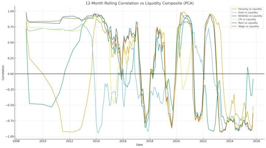
Compute rolling correlations between LCI-PCA and each asset on monthly data. Compare those correlations to rolling correlations between CPI proxies and the same assets. The expectation is not perfect correlation. The expectation is that liquidity correlations are stronger and more consistent across regimes.
Lead/lag testing
Compute lead/lag windows for LCI versus each asset (cross-correlation on monthly changes). Gold should show shorter lags. Housing should show longer lags. Equities often show reflexive behavior in both directions due to discounting and positioning.
Robustness checks
- Test LCI_EW vs LCI_PCA to confirm regime consistency.
- Run PCA on subperiods to ensure factor stability.
- Test sensitivity to standardization window.
- Document post-2024 correlation weakening as a transition signal and justify the STC extension.
If LCI explains 2003–2023 well but appears “less clean” post-2024, do not treat that as a model death. Treat it as a system upgrade. A new collateral channel is muting the old signal. That is exactly why STC exists in this paper.
Rebuild it yourself (spreadsheet or Python)
Reproducibility is non-negotiable. This is not a vibes model. The base factor can be rebuilt from public series in either a spreadsheet or Python.
Spreadsheet build
- Pull monthly WALCL, WTREGEN, RRPONTSYD, M2SL.
- Invert WTREGEN and RRPONTSYD.
- Z-score each series (use a consistent window).
- Compute equal-weight composite and chart.
- Optional: run PCA and anchor sign against the equal-weight composite.
Python build (outline)
# 1) Load monthly series for WALCL, WTREGEN, RRPONTSYD, M2SL
# 2) Invert drains: WTREGEN, RRPONTSYD
# 3) Z-score each
# 4) LCI_EW = mean(zscores)
# 5) PCA on zscores -> first component
# 6) Anchor sign: if corr(LCI_PCA_raw, LCI_EW) < 0: multiply by -1
# 7) Overlay on GOLDAMGBD228NLBM, NASDAQCOM, CSUSHPINSA
This is Tier-1. It tells you the macro regime. The next sections explain why, in a world of tokenized collateral and stablecoin rails, regime can remain risk-supportive even when people think “liquidity should be tight.”
Synthetic liquidity amplification (stablecoins + looping)
The four-reservoir model measures baseline liquidity. It explains regime shifts. But it does not fully describe the emerging reality where liquidity can be assembled outside classic QE channels through collateral wrappers, leverage loops, and rehypothecation stacks.
Substrate: front-end Treasuries (bills/repo/MMFs) as the base collateral.
Wrapper: stablecoins/tokenized T-bills that turn that collateral into portable reserve-like claims.
Multiplier: looping/rehypothecation that builds stacked claims on the same base.
Stablecoins are the interface. They convert short-duration Treasury collateral into programmable, transferable claims that can circulate continuously across systems. This changes velocity. Velocity changes leverage capacity. Leverage capacity changes pricing.
What stablecoins are in this framework
In this paper, stablecoins are treated as collateral wrappers around short-duration, high-quality liquid assets. The headline is not “crypto adoption.” The headline is that the short end is being converted into a mobile reserve substrate, and the system can build layered claims on top of it.
The first “loop” is not DeFi
The government already borrowed when it issued the T-bill. When that bill backs a stablecoin, the private sector has created an additional claim layer on the same collateral. That is the seed crystal. DeFi looping and rehypothecation come later, but the base layering starts the moment the bill becomes the reserve substrate for a transferable claim.
The Stablecoin Leverage Loop (text model)
The looping mechanism is simple and brutal: deposit collateral, borrow against it, redeposit the borrowed asset as new collateral, borrow again. Each iteration increases gross notional exposure while the base seed remains the same.
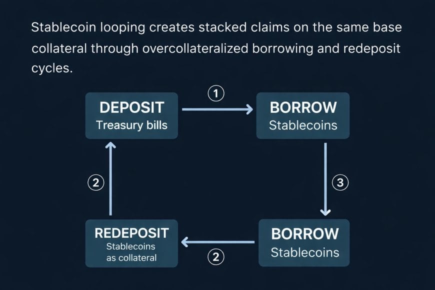
If effective LTV is r, the gross collateral multiplier is approximately 1/(1−r) when you recursively borrow and redeposit. At r=0.90, gross approaches ~10x. At r=0.95, gross approaches ~20x. Real-world realized multipliers are lower due to buffers, fees, utilization spikes, and liquidation headroom.
Why this is happening now
There are multiple converging drivers, and you only need a few of them for the system to scale:
- Collateral demand is global: the world wants dollar collateral that clears and settles fast.
- Front-end paper is the cleanest substrate: short-duration Treasuries behave like industrial-grade near-cash.
- Tokenization increases velocity: settlement speed and portability make the same base collateral “do more work.”
- Post-2022 lesson: collateral scarcity was a real stressor; the system learned that front-end collateral is king.
- Policy optics: synthetic liquidity channels are politically cleaner than overt QE messaging.
- Market structure: 24/7 venues plus automated liquidation engines increase transmission speed.
None of this requires retail users to be the dominant driver. Which leads to the mechanism most people miss: the institutional loop.
The fifth reservoir: STC (stablecoin/T-bill collateral)
Tier-1 LCI measures baseline liquidity. Tier-2 explains amplification. Tier-3 formalizes the new reservoir as a first-class variable: STC, Stablecoin Treasury Collateral.
STC represents Treasury bill collateral held inside stablecoin reserve structures, plus Treasury collateral that becomes token-eligible and collateral-eligible inside digital collateral programs. This reservoir matters because it can expand claim capacity even when baseline LCI is flat.
Define the base collateral universe (the $6T vs $9T argument)
People will attack your number if you don’t define the universe. So define it cleanly.
“T-bills outstanding” is one number. “Liquid rollable front-end collateral universe” is a broader definition: bills plus bill-backed repo capacity plus cash-management vehicles that concentrate into bills (money market funds) plus tokenizable short-duration Treasury exposure. This paper uses the broader universe when discussing “system capacity,” because the system does not operate on one accounting line item. It operates on the entire front-end collateral stack and its reuse pathways.
Three layers of STC
- STC₁ (Issuer layer): Treasury bills and bill-backed repo/MMFs held as reserves behind stablecoin supply.
- STC₂ (Market layer): tokenized short-duration Treasury products used as collateral in lending and margin systems.
- STC₃ (Institutional layer): banks, brokers, custodians, and collateral programs using stablecoins and tokenized Treasuries as settlement and margin substrate.
The bank-as-borrower mechanism (institutional loop)
This is the missing piece from most stablecoin explanations: you do not need retail loopers to build scale. Replace the borrower with a bank balance sheet and the machine becomes institutional.
Here is the clean pathway:
- Step 1: Bank A allocates cash to short-duration Treasuries (or bill-backed repo) as the base collateral.
- Step 2: Bank A uses a stablecoin rail (issuer partnership or internal issuance in a permitted structure) to create a transferable claim against that collateral.
- Step 3: Bank A lends the stablecoin as a settlement/margin asset into a network that accepts it as near-cash.
- Step 4: The stablecoin becomes the “cash leg” used to acquire additional Treasury exposure (directly, through tokenized T-bill products, or through collateral programs).
- Step 5: The system reinforces front-end demand while building a layered claim stack above the same base substrate.
That is not “DeFi leverage.” That is a modernized repo-style engine expressed through tokens and collateral eligibility rules.
STC proxy (measurable, even if imperfect)
STC is not one clean public series. So treat it like a macro composite: use a proxy set, standardize it, and track its trend and acceleration.
STC_proxy(t) =
  z(Stablecoin_Total_Supply) +
  z(Stablecoin_Dominance_Concentration) +
  z(Estimated_Treasury_Share_in_Reserves) +
  z(Tokenized_TBill_And_MMFloat_OnChain) +
  z(Collateral_Eligibility_Signals)
Then you can either (1) overlay STC_proxy on LCI-PCA as a second axis, or (2) include it as a fifth input for a post-2024 “LCI5” factor, while keeping the original LCI-PCA intact for historical continuity.
LCI5_PCA(t) = PCA1(
  z(WALCL),
  z(-TGA),
  z(-RRP),
  z(M2),
  z(STC_proxy)
)LCI explains the baseline liquidity climate. STC explains collateral velocity and claim capacity. When LCI is flat but STC is rising, “everything up” regimes can appear without classic QE signals.
Sizing the leverage envelope (how the front end becomes a claim engine)
This is where people get emotional and start fighting the wrong argument. The question is not “are stablecoins literally printing dollars.” The question is: how large can the claim stack become when the base substrate is multi-trillion front-end collateral and the system is allowed to wrap it, move it, and reuse it.
Separate the three multipliers (do not mix them)
- Multiplier A (roll mechanics): bills mature and are reinvested continuously; not leverage, just persistent allocation.
- Multiplier B (recursion): deposit, borrow, redeposit; creates gross notional footprint above the base.
- Multiplier C (rehypothecation): hidden reuse via netting/substitution; expands effective claim capacity without a visible single loop.
The clean sizing model (bounded, not fantasy)
- S = total stablecoin supply
- f = fraction that enters leverage/collateral reuse venues
- m = effective realized multiplier (buffers + costs included)
Gross notional footprint ≈ S × f × mIf S = $1T stablecoin supply, and f = 30% actually enters leverage/reuse venues, and realized m = 4x, then gross footprint ≈ $1T × 0.30 × 4 = $1.2T. The headline numbers only explode when participation rates and realized multipliers move from “small niche” to “systemic adoption.”
The constraint is not token minting. The constraint is confidence, redemption liquidity, market depth, collateral eligibility, and liquidation speed. When those are stable, claim capacity expands quietly. When one fails, the unwind compresses fast.
Why the front end gets bid
If you only view T-bills as “yield,” you miss the trade. The short end is increasingly being treated as substrate: the raw material for a collateral stack that can be wrapped and reused.
There are structural reasons the bid concentrates at the front end:
- Redemption design: a stable reserve set must survive redemption waves, so it hugs very short duration.
- Collateral cleanliness: front-end Treasuries and bill-backed repo are the cleanest form of “cash-like” collateral.
- Roll dynamics: short duration means constant maturity events; reserves can be continuously refreshed without duration shocks.
- Funding logic: if collateral is the system’s operating system, the front end is the kernel.
And there is a macro reality: large pools of cash already exist that want front-end instruments, and they can absorb large issuance. That is why the “front end as infrastructure” framing is not rhetorical. It is an allocation outcome.
Failure modes: how this unwinds
The stablecoin collateral layer adds capacity. It also adds new unwind paths. Unwinds can occur faster than traditional systems because liquidation engines and redemption flows are more automated. The expansion can be quiet. The unwind can be violent.
A realistic unwind sequence (speed is the variable)
- Confidence shock: regulatory headline, counterparty fear, collateral event, or narrative fracture.
- Redemption pressure: holders rush for cash; issuer liquidity buffers get tested.
- Reserve mobilization: bills/repo are sold or financed; the front end feels it.
- Venue tightening: borrow rates spike, LTVs are cut, eligibility tightens.
- Liquidation cascades: stacked claims unwind mechanically and quickly.
- Synthetic liquidity collapses: the claim stack compresses; risk reprices; tape flips.
Failure Mode A: issuer redemption wave
If confidence drops, holders redeem. Issuers must meet redemptions with cash and near-cash. If redemptions exceed liquidity buffers, reserve assets are liquidated or repo’d. Stress transmits into the front end.
Failure Mode B: liquidation spiral
Looping creates stacked claims. If collateral values slip or borrow rates spike and positions become unhealthy, liquidations accelerate. Liquidations can overwhelm market depth before humans react.
Failure Mode C: collateral eligibility shock
If a major venue changes collateral rules, the system can delever overnight. Eligibility is not a detail. It is a control lever.
Failure Mode D: “policy perimeter” shock
Stablecoins live at the intersection of money, payments, and collateral. A rapid regulatory shift can force reserve reallocation and risk compression even without a market catalyst.
The system can expand quietly and unwind violently. Not because it is “fake.” Because it is faster than the old system.
What it means (regimes, policy, and hard assets)
This is the stacked conclusion.
Tier-1 LCI remains the baseline regime factor. It explains why hard assets reprice across cycles: expanding liquidity expands the collateral stack’s ability to carry risk.
Tier-2 amplification explains why liquidity can appear without classic QE. The system can assemble synthetic liquidity through collateral wrappers, looping, and rehypothecation. This can produce “everything up” conditions even when the lived economy remains tight and political discourse stays bearish.
Tier-3 STC explains why the dollar’s future is not only currency dominance but collateral dominance. If the global system adopts tokenized dollar collateral at scale, the dollar becomes a reserve operating system: a standardized substrate for settlement, margin, and collateral reuse.
Regime signature: “everything up, including the dollar”
Classic thinking says a strong dollar should tighten financial conditions and cap risk. That relationship can weaken when the dollar is the collateral base being demanded and when collateral velocity is rising. In that regime, USD strength and asset inflation can coexist because the collateral economy is bidding the reserve substrate while also bidding convexity on top of it.
How this connects back to hard assets
Hard assets follow liquidity because liquidity is the governing variable of the collateral economy. The only change is that liquidity is now assembled from multiple layers, not solely from the Fed balance sheet. If you are looking at CPI and wondering why gold or housing behaves “wrong,” you are watching the wrong machine.
Pattern Nexus Lens
The simplest interpretation is the most uncomfortable: the system is evolving into a two-tier dollar.
Tier one is the visible dollar: wages, prices, CPI, politics. Tier two is the collateral dollar: Treasury bills as substrate, stablecoins as wrappers, and leverage venues as multipliers. Hard assets price the second tier.
QE was the visible era. Collateral assembly is the next era. The front end is the substrate. Stablecoins are the interface. Rehypothecation and looping are the multiplier. Hard assets respond accordingly.
Liquidity is not only printed. It is assembled. When the assembly line runs, hard assets reprice. When the assembly line reverses, synthetic liquidity becomes synthetic illiquidity faster than most models assume.
FAQ
Is LCI a trading signal?
No. LCI is a regime factor. It identifies expansion, plateau, constriction, and bottom conditions. It is designed for macro horizon alignment, not weekly prediction.
Why add stablecoins if LCI already works?
Because the transmission mechanism is changing. LCI explains baseline liquidity conditions. Stablecoins and tokenized collateral explain a new amplification layer that can expand claim capacity outside classic QE framing.
Does this imply infinite money?
No. It implies layered claims and synthetic liquidity capacity. The system still faces constraints: redemption liquidity, market depth, collateral eligibility, and liquidation mechanics.
What number matters most going forward?
Watch the combination of baseline liquidity (LCI) and collateral layer expansion (STC proxies). When both rise, hard assets tend to reprice aggressively. When LCI falls and the STC layer compresses, risk reprices fast.
What is the most common misunderstanding of the stablecoin layer?
That the reserve layer is the entire story. The reserve layer is the base. The expansion happens when the stablecoin becomes collateral, becomes margin, and enters leverage and rehypothecation systems. That is where the claim stack grows.
Sources
Public series and primary references used for the baseline LCI build and the STC collateral extension.
- FRED: WALCL — Federal Reserve Total Assets
- FRED: WTREGEN — Treasury General Account
- FRED: RRPONTSYD — Overnight Reverse Repo
- FRED: M2SL — M2 Money Stock
- FRED: CSUSHPINSA — Case-Shiller National Home Price Index
- FRED: GOLDAMGBD228NLBM — LBMA AM Gold Price
- FRED: NASDAQCOM — NASDAQ Composite Index
- DefiLlama: Stablecoin market cap and dominance
- U.S. Treasury Fiscal Data: Monthly Statement of the Public Debt (MSPD)
- GovInfo: Public Law 119–27 (GENIUS Act) landing page
- Reuters: money market funds absorbing T-bill supply
- Financial Times: Fed reserve management bill purchase framing (late 2025)
What's Your Reaction?
 Like
0
Like
0
 Dislike
0
Dislike
0
 Love
0
Love
0
 Funny
0
Funny
0
 Wow
0
Wow
0
 Sad
0
Sad
0
 Angry
0
Angry
0

Founder of Pattern Nexus. I research markets, macro, geopolitics, AI, history, ancient systems, and the patterns most people overlook. I’m also building Market Radar, a trading scanner designed to read pressure, risk, confirmation, and setup quality before chasing a move. Pattern Nexus is where I connect the dots between data, history, technology, and the bigger system playing out around us.
















Comments (1)