

Hard Assets Follow Liquidity, Not Inflation? The Full Data Reconstruction — 2026 Update
A 2003–2026 reconstruction of Fed liquidity, gold, housing and NASDAQ data, plus an experimental stablecoin-augmented liquidity index. Meta tags: liquidity conditions index, hard assets, gold, Federal Reserve balance sheet, Treasury General Account, reverse repo, M2, stablecoins, tokenized Treasuries, housing, NASDAQ, PCA


What the full reconstruction actually establishes
- The original insight survives, but the absolute wording does not. Gold, technology shares and housing are priced inside a capital system shaped by money, collateral, funding capacity, discount rates and credit. That makes liquidity indispensable. It does not make inflation, wages, rents, supply, earnings or valuation irrelevant.
- The historical model is preserved before it is challenged. LCI4 remains the sign-anchored first principal component of Federal Reserve assets, an inverted Treasury General Account, an inverted overnight reverse-repo balance and M2. The closed calibration sample contains 281 month-end observations from February 2003 through June 2026.
- July is a live snapshot, not a completed month. Observations available through July 26 are projected through parameters fitted only through June. M2 still refers to May and Case-Shiller still refers to April, so the July row is useful for monitoring but not a synchronized final observation.
- Gold has been rebuilt from a different provider across the full sample. This edition uses the World Bank Pink Sheet monthly average for every month, rather than splicing a new source onto the old Fed-hosted London fixing series. The latest closed gold observation is $4,228 per troy ounce for June 2026.
- The long-run level relationships remain large. LCI4 correlates 0.701 with gold, 0.854 with the NASDAQ Composite and 0.875 with the national Case-Shiller index in levels. Those charts retain the visual force of the original thesis.
- The stricter tests are much weaker. Correlations between monthly changes in LCI4 and monthly asset returns are −0.005 for gold, −0.107 for NASDAQ and +0.053 for housing. Rolling relationships move through positive and negative regimes. LCI4 is therefore a descriptive regime factor, not a mechanical monthly trading signal.
- The PCA continuity series and the economic-direction audit disagree at the current endpoint. LCI4 falls from 1.27 standard deviations in June to 1.20 in the partial July row, while the equal-weight four-input audit rises from 0.414 to 0.485. That divergence follows directly from PCA assigning negative loadings to the already-inverted TGA and RRP inputs and must be visible in any responsible interpretation.
- Stablecoin adoption is now large enough to monitor but too young to treat as causal proof. The extracted DefiLlama snapshot contains $306.8 billion of USD-pegged circulating value as of July 26. A five-input LCI5 improves all three in-sample level correlations over the shared November 2017–June 2026 window, but the improvement occurs inside a short, strongly trending sample.
- The current regime is split. The stock of money and tokenized-dollar claims remains historically large; ON RRP is almost exhausted; the TGA remains elevated; stablecoin supply is up over twelve months but down over the latest one- and three-month comparisons; and the two versions of the four-input composite point in different marginal directions.
- The title should be read as a research question. “Liquidity, not inflation” is a useful challenge to consumer-only explanations of asset prices. The updated evidence supports “liquidity as a first-order regime input,” not “liquidity as the only driver.”
The article, the model and the audit trail are one product
This edition does not simply extend the endpoint on an existing chart. It reconstructs the original argument section by section; preserves the four-input continuity model; documents the exact data vintages, units, frequencies and transformations; replaces the discontinued gold route without hiding the measurement change; publishes the fitted PCA loadings; separates a closed sample from the live month; tests levels, changes, rolling windows and leads or lags; and adds stablecoin adoption without inventing a pre-history.
It also restores the material that became fragmented across earlier drafts: the Colombo-chart question, the four-phase cycle, the response hierarchy, the 2003–2026 regime chronology, the practical tracking method, the real-economy translation, the stakeholder implications, the countercase, the falsification standard, the limitations and the complete source architecture. The original thesis is not silently discarded when the new data disagrees with it. Each major original claim is retained, tested and given an explicit 2026 verdict.
The downloadable package contains the raw provider files, the closed and live monthly panels, the transformed inputs, LCI4 and LCI5 outputs, the equal-weight audit series, fitted loadings, correlations, rolling diagnostics, lead-lag results, freshness flags, validation checks, all 31 source chart files, a formatted workbook, a source manifest and SHA-256 checksums.
Premium standard: a reader should be able to distinguish a measured fact from a model output, a mechanism from a correlation, a closed observation from a carried value, and a durable conclusion from a provisional interpretation.
Hard assets do not follow one variable. They move inside a connected system of money, collateral, discount rates, credit capacity, scarcity, cash flows and expectations.
The original Pattern Nexus thesis identified an important category error: a capital asset cannot be fully valued by comparing it only with CPI, current rent or current wages. Housing is simultaneously shelter, collateral and a leveraged long-duration asset. Gold is a monetary commodity whose opportunity cost depends heavily on real rates and confidence in sovereign claims. The NASDAQ Composite is an equity index whose value depends on distant earnings, discount rates and risk capacity. Each belongs to the capital system as well as the lived economy.
The rebuilt data continues to show strong long-run alignment between these assets and the balance-sheet variables condensed into LCI4. But the updated evidence also rejects the strongest version of the slogan. Standardizing trending levels does not remove their trends. PCA does not identify causality. The fitted component does not preserve every intended economic sign. CPI levels correlate even more strongly with the three asset-price levels in this sample. Monthly-change relationships are weak. Rolling correlations reverse. Leads and lags are small and unstable.
The result is not that liquidity “does not matter.” The result is a more useful hierarchy of claims. Liquidity is a first-order pricing environment because it shapes the ease of refinancing, the quantity and composition of money-like claims, the discount rate applied to future cash flows, the capacity to leverage collateral and the willingness to hold duration. Inflation is a separate first-order environment because it shapes real returns, nominal incomes, policy responses, replacement costs and the purchasing power of the unit in which assets are quoted.
The stablecoin extension reinforces the systems view. Tokenized dollars add a programmable settlement rail and create a new link between cash, Treasury collateral, exchanges, payments and on-chain leverage. Yet stablecoin issuance often transforms an existing deposit or Treasury-backed claim rather than creating a wholly new net dollar. Adoption scale is therefore economically relevant without being equivalent to bank reserves, M2 or transaction velocity.
Audited thesis: liquidity is upstream of many asset-price regimes, but it is not a universal timer or a complete valuation model. The practical edge comes from combining liquidity stock, liquidity direction, component composition, data freshness and asset-specific confirmation.
Contents
- The original question and the 2026 evidence boundary
- Source audit, data vintages and monthly alignment
- Reconstructing LCI4 and confronting the PCA sign problem
- The four traditional liquidity channels
- Gold, NASDAQ and housing versus LCI4
- Gold against each liquidity component
- NASDAQ against each liquidity component
- Housing, the Colombo comparison and affordability
- Levels, changes and rolling correlations
- Lead-lag tests and the causality boundary
- The original four-phase liquidity cycle revisited
- The hard-asset response hierarchy revisited
- Stablecoin adoption and the experimental LCI5
- The July 2026 operating dashboard
- What the reconstruction means for different stakeholders
- How to track and reproduce the framework
- What would strengthen or falsify the thesis
- Limitations, edge cases and failure modes
- The Pattern Nexus lens and final judgment
- The complete downloadable reconstruction
- Frequently asked questions
- Research and data sources
The missing variable was real; the original certainty was not
The original article began with a familiar viral comparison: national home prices had risen much faster than consumer prices, rents and wages. The visual implication was that housing had detached from the household economy and therefore represented a bubble waiting to mean-revert. Pattern Nexus challenged the conclusion by identifying a category mismatch. A house is not only a consumer service. It is also a scarce, financeable, tax-advantaged capital asset that serves as collateral.
That challenge remains important. A current wage or rent series does not contain the mortgage rate, loan-to-value constraint, duration of financing, tax treatment, construction pipeline, local land constraint, existing-home inventory, household balance sheet or marginal buyer’s cost of capital. Comparing a capitalized asset price with a current flow variable can reveal affordability stress without providing a complete valuation model.
The original article then moved from that valid critique to a much stronger universal claim: housing, gold and NASDAQ do not follow inflation, rents or wages; they follow liquidity. It described the pattern as predictable, mathematical, mechanical and nearly perfect. It called LCI-PCA the “true underlying driver,” treated rolling correlations as causal proof, declared that the housing-bubble argument collapsed and forecast a forced 2026 liquidity expansion.
The purpose of this update is not to erase that argument. It is to test every layer of it with the longer sample and preserve a clear boundary between what survives and what does not.
- Consumer layer
CPI, rent and wages describe prices, income and lived affordability. - Capital layer
Discount rates, leverage, collateral, cash flows and scarcity shape asset capitalization. - Plumbing layer
Fed assets, Treasury cash, reverse repos and M2 describe different monetary and funding channels. - Digital-dollar layer
Stablecoins and tokenized Treasuries extend settlement and collateral onto programmable rails. - Evidence layer
Levels, changes, rolling windows and lead-lag tests answer different statistical questions.
Definitions that prevent the argument from collapsing into slogans
Inflation is a rate of change in a price index. The level of CPI is the cumulative price index; its monthly or annual change is the inflation rate. A correlation between the CPI level and an asset-price level is not the same statistic as a correlation between inflation and an asset return.
Liquidity has no single universally accepted market series. In this article it means a set of balance-sheet and money-stock conditions that may influence deployable funding, refinancing capacity, collateral demand and portfolio substitution. LCI4 is one statistical compression of four chosen proxies. It is not “all liquidity.”
Hard asset is used as a research shorthand. Gold and housing fit the conventional definition more closely than the NASDAQ Composite. NASDAQ is included because long-duration growth equities are highly sensitive to discount rates and risk capacity, which makes the index a useful cross-asset test of the liquidity hypothesis.
Following can mean at least four different things: sharing a long-run trend, moving contemporaneously, responding after a lag or being caused by a prior change. The original article often moved among these meanings. This update measures them separately.
The original claim audit
| Original proposition | 2026 assessment | Audited conclusion |
|---|---|---|
| Capital assets cannot be explained by consumer variables alone | Supported | Affordability variables are essential, but they are not a complete capitalization model. |
| WALCL, TGA, RRP and M2 form an interacting system | Supported as a framework | The four channels represent different balance sheets and should be examined jointly and separately. |
| LCI-PCA is the “true” liquidity factor | Overstated | PCA1 is the dominant in-sample covariance factor. Its negative loadings on already-inverted TGA and RRP prevent it from being treated as a mechanically liquidity-positive structural index. |
| Housing follows liquidity, not CPI, rent or wages | Too absolute | Housing has a strong LCI4 level relationship, but CPI has an even higher level and monthly-change correlation in this sample. Mortgage structure, income and supply also matter. |
| Gold responds fastest | Not established as a fixed rule | Gold can reprice rapidly, but the tested LCI4 lead correlations are small and unstable. |
| NASDAQ is the purest liquidity expression | Partly supported, not universal | NASDAQ has a high LCI4 level correlation and the highest M2 component correlation, but earnings and the current technology investment cycle create large independent moves. |
| Housing is the slowest consistent follower | Mechanically plausible, statistically weak | The best LCI4 positive-lag change correlation with housing is only 0.125 at twelve months. |
| Rolling hard-asset correlations remain near +0.8 to +1.0 | Contradicted | Twelve-month level correlations repeatedly travel from strongly positive to strongly negative. |
| The four-phase cycle explains every major move | Useful taxonomy, not a law | Expansion, plateau, constriction and repair are helpful regime labels, but the fitted PCA series is trend-dominated and does not recover a clean repeating oscillator. |
| A forced 2026 liquidity expansion is inevitable | Not supported | The July dashboard is mixed. RRP is exhausted and M2 is high, while TGA is elevated, Fed assets remain below their peak and the PCA and equal-weight composites disagree on the latest direction. |
Evidence boundary: the update preserves the capital-system insight and rejects the claim that one composite explains everything. That is a stronger research product because it tells readers where the framework is informative and where another variable must carry the analysis.
One closed sample, one live snapshot and explicit publication lag
The closed analytical sample contains 281 month-end observations from February 2003 through June 2026. All full-sample means, population standard deviations, PCA loadings, level correlations, monthly-change correlations and rolling diagnostics are estimated from those closed rows. The July 31 row is a live period bucket constructed from data available through July 26. It is projected through the June-fitted parameters and excluded from estimation.
This distinction is indispensable because the inputs do not arrive on the same schedule. A daily equity index can be current through the prior trading day while a national home-price index still describes transactions from three months earlier. A chart can place both values in a July row only by carrying the last available housing observation forward. That alignment is convenient, but the carried value is not new information.
| Series | Exact measurement | Latest raw period or date | Latest value | Provider |
|---|---|---|---|---|
| WALCL | Federal Reserve total assets, Wednesday level; weekly; millions of dollars | July 22, 2026 | $6.747T | Federal Reserve via FRED[4] |
| WTREGEN | Treasury General Account, week average ending Wednesday; millions of dollars | July 22, 2026 | $829.6B | Federal Reserve via FRED[5] |
| RRPONTSYD | Overnight reverse-repo daily amount; billions of dollars | July 24, 2026 | $0.675B | New York Fed via FRED[6] |
| M2SL | M2 money stock; monthly; seasonally adjusted; billions of dollars | May 2026 | $23.052T | Federal Reserve via FRED[7] |
| CSUSHPINSA | S&P Cotality Case-Shiller U.S. National Home Price Index; monthly; not seasonally adjusted | April 2026 | 332.678 | S&P Dow Jones Indices via FRED[8] |
| NASDAQCOM | NASDAQ Composite daily close | July 24, 2026 | 24,975.82 | NASDAQ via FRED[9] |
| CPIAUCSL | Consumer Price Index for All Urban Consumers; monthly; seasonally adjusted | June 2026 | 332.568 | BLS via FRED[10] |
| CUUR0000SEHA | CPI for rent of primary residence; monthly; not seasonally adjusted; 1982–1984 = 100 | June 2026 | 446.945 | BLS via FRED[11] |
| AHETPI | Average hourly earnings of production and nonsupervisory private employees; monthly; seasonally adjusted | June 2026 | $32.38/hour | BLS via FRED[12] |
| Gold | Monthly average spot price; dollars per troy ounce | June 2026 | $4,228 | World Bank Pink Sheet[13] |
| USD stablecoins | Total USD-pegged circulating value in the extracted daily API series | July 26, 2026 | $306.757B | DefiLlama[14] |
| Tokenized Treasuries | Distributed value in the retrieved point-in-time dashboard snapshot | July 26, 2026 | $16.197B | RWA.xyz[15] |
Corrections made during the audit
- Gold is a full-sample replacement, not a splice. Every monthly gold observation used in this edition comes from the World Bank file. The measurement differs from the prior London fixing route across editions, but there is no provider break inside the reconstructed 2003–2026 series.
- AHETPI is not the all-employees series. It measures production and nonsupervisory employees in total private employment. That distinction is now stated correctly in the article, source manifest, processed observation table and workbook.
- The rent index base is 1982–1984 = 100. The prior metadata label of December 1997 = 100 was incorrect and has been corrected.
- Case-Shiller’s current provider branding is Cotality. “CoreLogic” describes the earlier brand associated with the same national index but is not the current FRED title.
- WTREGEN is a weekly average. The July 22 observation is not a single point-in-time Treasury cash balance. Treating it as a week average matters when comparing it with a daily market close.
- Provider dashboards can change after extraction. The article and workbook use the values preserved at the July 26 cutoff. A live webpage viewed later can show a revised value, a different coverage definition or a newer update.
Monthly alignment rules
- For daily and weekly data, retain the last non-missing observation available within each calendar month.
- For monthly data, place the published period into its month-end bucket.
- Forward-fill release gaps so all columns can be compared on a common month-end index, while recording the age of the carried observation in a separate freshness table.
- Set only genuine RRP pre-history to zero. Do not replace ordinary missing observations in other series with zero.
- Leave stablecoin pre-history blank. A technology that was not yet measured cannot be assigned a fabricated zero history merely to extend the PCA sample.
- Estimate all model parameters on closed rows through June 2026, then project the July live row through those fixed parameters.
At the June endpoint, M2 is carried one month and Case-Shiller is carried two months. At the live July endpoint, those publication lags become two and three months. CPI, rent CPI, hourly earnings and gold are carried one month into July. WALCL, TGA, RRP, NASDAQ and stablecoins have July observations, but they do not share one timestamp.
What “full-sample” means for interpretation
The z-scores use the mean and population standard deviation of the entire February 2003–June 2026 sample. This makes the historical chart internally comparable and reproduces the established Pattern Nexus method. It also means an early-period z-score uses information that would not have been available in real time. The model is a retrospective reconstruction, not a vintage-by-vintage backtest.
FRED and other providers can revise historical data. The package preserves the downloaded files and their hashes, but it is not an archive of every value as originally released. A true real-time forecasting test would require vintage data and a rolling or expanding estimation window.
Reproducibility rule: “current” always means current as of an explicit extraction cutoff. In this edition that cutoff is July 26, 2026. It does not mean that every underlying economic period is July or that the values will remain unchanged on the provider’s website.
The continuity model is preserved—and its internal contradiction is made explicit
The original four-input specification first places each variable in an intended economic direction:
Inputs = WALCL, −TGA, −RRP, M2
A larger Federal Reserve balance sheet and a larger M2 stock are defined as more supportive. A larger Treasury cash balance and a larger reverse-repo balance are defined as drains, so their signs are inverted before standardization. For each transformed input x, the model calculates:
z(x) = [x − full-sample mean(x)] ÷ full-sample population standard deviation(x)
This step is necessary because the raw series use different units and scales. WALCL and TGA are reported in millions of dollars, RRP and M2 in billions, and their typical variations differ by orders of magnitude. Standardization makes them dimensionless. It does not make them economically equivalent and does not remove long-run trends.
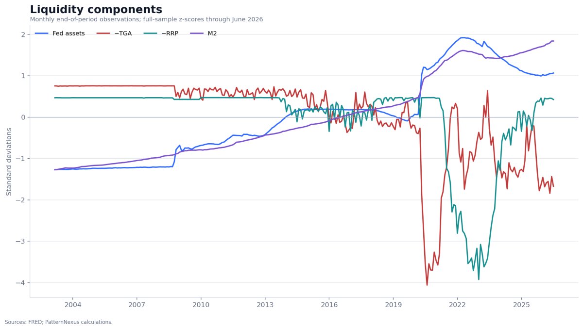
The component chart demonstrates why “liquidity” cannot be inferred from one pipe. In 2020, Fed assets and M2 moved sharply higher, while Treasury cash also accumulated and the reverse-repo facility later expanded dramatically. Some channels added balance-sheet capacity while others absorbed or redirected cash. The net market effect depended on counterparties, collateral, issuance, regulation and risk appetite.
Principal component analysis then finds the linear combination of the four standardized inputs that explains the largest share of their joint in-sample variance. PCA does not know the economic interpretation of a Treasury drain or a reverse-repo balance. It simply finds a covariance direction.
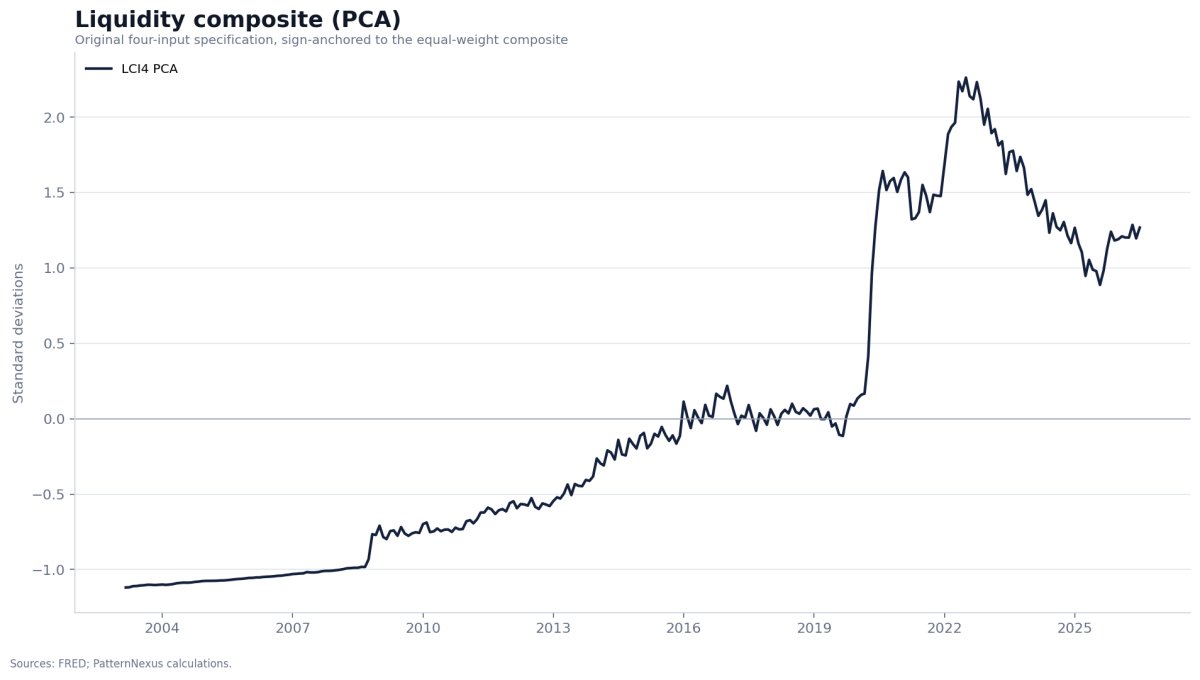
The first component explains 76.47% of the standardized input variance. That is enough to say the four columns contain a dominant shared statistical direction. It is not enough to say the component is a structural causal measure of “net liquidity.”
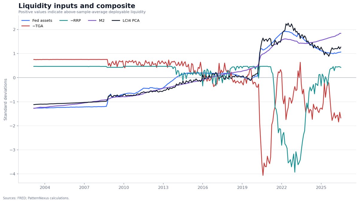
The sign anchor solves one problem, not every sign problem
A PCA component can be multiplied by −1 without changing its statistical validity. The established Pattern Nexus method resolves that sign indeterminacy by comparing PCA1 with the equal-weight average of the four economically directed z-scores and flipping the whole component when the correlation is negative. After anchoring, a higher overall PCA score is intended to mean easier liquidity.
That procedure determines the sign of the component as a whole. It does not force each fitted loading to agree with the economic sign assigned before PCA. In this sample, the loadings are:
| LCI4 input | Pre-PCA economic direction | PCA1 loading | Interpretation |
|---|---|---|---|
| WALCL | Higher = easier | +0.562 | Agrees with the intended direction |
| −TGA | Higher = easier | −0.462 | Opposes the intended direction inside PCA1 |
| −RRP | Higher = easier | −0.405 | Opposes the intended direction inside PCA1 |
| M2 | Higher = easier | +0.555 | Agrees with the intended direction |
The anchored PCA score correlates only 0.486 with the equal-weight audit series over the closed sample. The correlation is positive, so the global sign rule passes. It is not close enough to treat the two measures as interchangeable. The PCA factor is best described as the historical continuity factor dominated by the shared WALCL and M2 trend. The equal-weight series is the cleaner audit of the pre-imposed “all easier inputs raise the index” logic.
The current endpoint exposes the issue
From the June closed row to the July live row, the TGA falls from $918.7 billion to $829.6 billion and ON RRP falls from $26.9 billion to $0.675 billion. Under the conceptual signs, both movements are liquidity-positive. Fed assets also rise modestly, while the latest published M2 value is carried unchanged.
The equal-weight audit therefore rises from 0.414 to 0.485. The PCA continuity series falls from 1.268 to 1.197 because the fitted negative loadings on the already-inverted TGA and RRP turn those conceptually easier moves into negative PCA contributions. That is not a software error. It is the direct output of an unconstrained statistical method.
This distinction changes how the dashboard must be written. “LCI4 is falling” is true for the historical PCA series. “The four conceptual pipes tightened in July” is not. A responsible interpretation reports both.
Model-governance rule: preserve LCI4-PCA for continuity, but never use it alone when the fitted loading signs oppose the model’s economic direction. Review the equal-weight audit and the four components beside it. A future production model should test constrained weights, rolling estimation and out-of-sample stability.
Four channels feed, drain or redirect the same financial system
The original article described WALCL, TGA, RRP and M2 as a four-body system. That remains the right intuition, provided the metaphor does not imply that every dollar has the same transmission. A reserve balance at the Federal Reserve, a Treasury deposit, a money-fund reverse-repo claim and a household bank deposit sit on different balance sheets. They have different counterparties, legal forms, velocities and collateral uses.
The useful question is not simply whether each line is rising or falling. It is who holds the claim, what asset or liability changes on the other side, whether private balance-sheet capacity expands and where the marginal holder can redeploy the proceeds.
Federal Reserve assets: the baseline balance-sheet channel
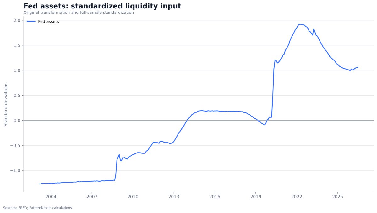
When the Federal Reserve purchases securities, it generally credits reserve balances in the banking system. That can remove duration or credit risk from private portfolios, alter the supply of safe collateral, support market functioning and lower term or liquidity premia. The effect on asset prices depends on what sellers and intermediaries do next. Reserves are not a bag of cash that leaves a bank and directly purchases a house or a share of stock.
WALCL is therefore a useful measure of central-bank balance-sheet scale, not a complete measure of financial ease. A large balance sheet can coexist with restrictive policy rates, weak bank lending, wider credit spreads or tighter dealer intermediation. Conversely, private credit and fiscal flows can support asset demand while WALCL is flat or declining.
The standardized level has a 0.703 correlation with gold, 0.828 with NASDAQ and 0.825 with Case-Shiller over the closed sample. The monthly-change correlations are −0.056, −0.036 and +0.062. The level alignment is meaningful as a regime observation; the short-run relationship is weak.
The Treasury General Account: fiscal cash timing inside monetary plumbing
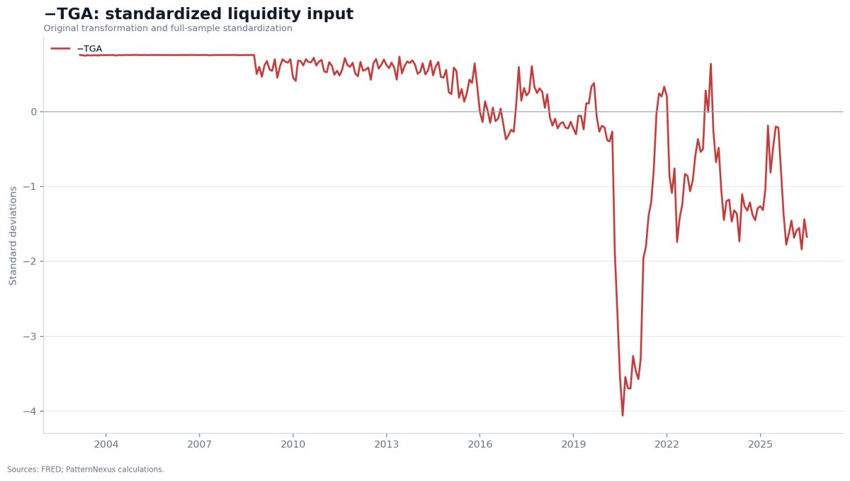
The TGA is the Treasury’s deposit account at the Federal Reserve. When taxes or debt issuance move funds into the account, private bank deposits or reserve balances can decline, depending on the purchaser and settlement path. When Treasury spends, its payment can return deposits and reserves to the private system. That is why the raw TGA is inverted in the conceptual model.
But the shorthand “TGA down equals liquidity up” omits the financing context. A spend-down funded by prior bill issuance differs from deficit spending accompanied by new issuance. Bill supply can pull money from ON RRP, deposits or other assets. Treasury payments can land in sectors with different propensities to spend, save or buy financial assets. The maturity mix of issuance affects collateral availability and dealer balance sheets.
The TGA comparison is also one of the clearest challenges to a universal one-pipe story. The inverted TGA level correlates −0.624 with gold, −0.741 with NASDAQ and −0.686 with Case-Shiller. The corresponding monthly-change correlations are −0.064, +0.036 and +0.053. TGA flows matter operationally, but these full-sample statistics do not support a stable, proportional asset-price rule.
Overnight reverse repo: a cash buffer that has nearly disappeared
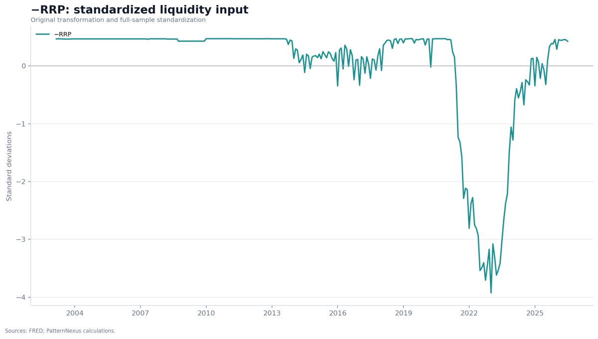
In a reverse-repo transaction, an eligible counterparty places cash with the Federal Reserve and receives securities with an agreement to reverse the transaction. The New York Fed describes temporary reverse repos as operations that drain reserves from the banking system and influence money-market conditions.[18] In the post-2021 regime, money-market funds used the overnight facility as a safe investment outlet.
When ON RRP declines, a money fund replaces a Federal Reserve claim with another short-term claim—often a Treasury bill, repo or similar instrument. That can ease specific funding or collateral conditions, but it does not guarantee that the same dollar purchases a risky asset. The transaction may remain entirely inside the safe-asset complex.
The near-exhaustion of the facility has two opposite interpretations. A low stock is supportive relative to the period when more than $2 trillion was parked at the Fed. But there is little remaining balance to drain, so the cushion that offset other forms of tightening cannot repeat at the same scale.
The inverted RRP level correlates −0.232 with gold, −0.418 with NASDAQ and −0.594 with Case-Shiller. Monthly-change correlations are +0.093, +0.133 and −0.135. These signs vary by asset and transformation. RRP should be treated as a conditional funding buffer, not a universal risk-asset valve.
M2: the slow structural stock with the strongest component-level alignment
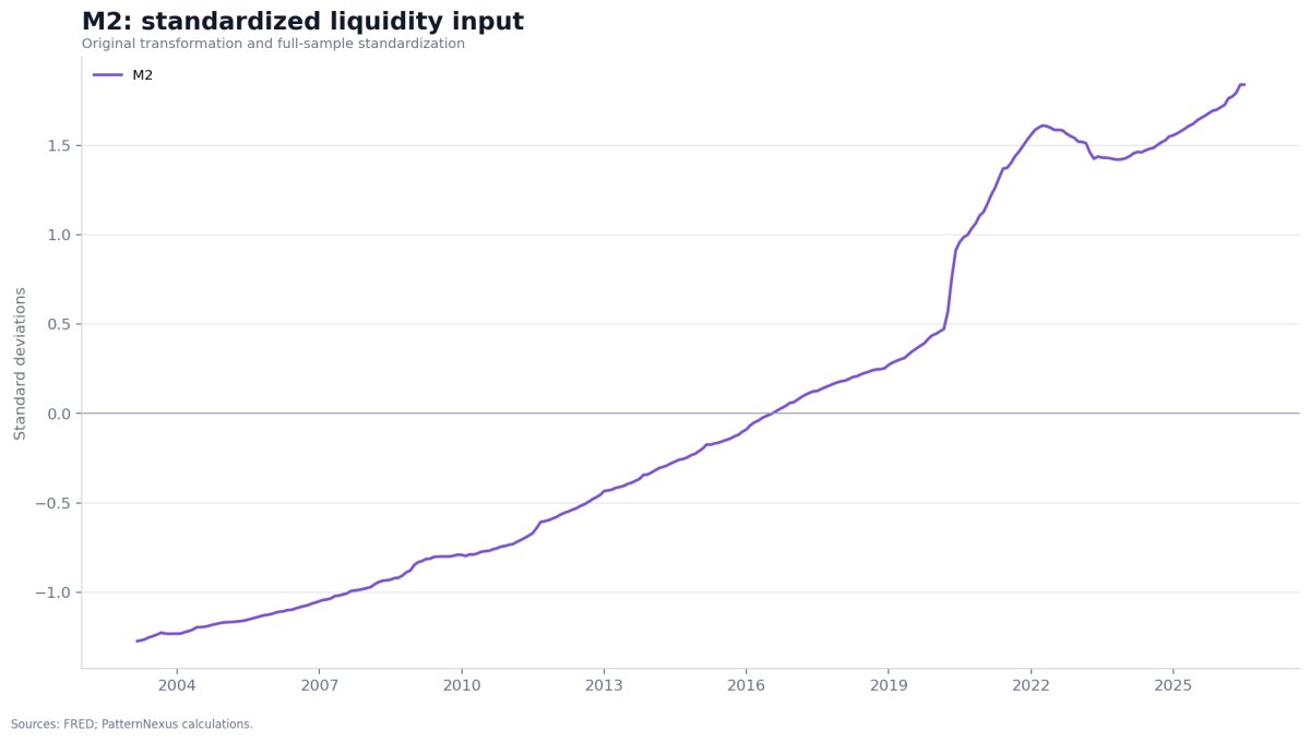
M2 includes currency, deposits and selected retail money-market balances. It is much closer than WALCL to the money balances held by households and firms, but it still says nothing directly about who owns the balance, how quickly it turns over, whether it is pledged or idle, or whether a marginal dollar is used for consumption, debt repayment or asset purchases.
The Federal Reserve’s M2 definition also changed beginning in May 2020 when the regulatory treatment of savings deposits changed and “other liquid deposits” moved into M1. FRED documents the before-and-after definitions on the series page.[7] That does not make M2 unusable, but it is another reason to resist treating a smooth chart as a timeless structural law.
M2 has the strongest component-level correlation with all three asset-price levels: 0.809 with gold, 0.934 with NASDAQ and 0.918 with Case-Shiller. Monthly-change correlations are only +0.064, +0.118 and +0.113. The difference is central to the entire reconstruction. M2 and nominal asset prices share a powerful long-run monetary and time trend. Their month-to-month innovations share much less.
Component conclusion: the four series describe different parts of the dollar system. Their combined reading is more informative than any one pipe, but statistical aggregation cannot erase the different mechanisms or guarantee a common multiplier.
The same continuity factor produces three different economic stories
The first asset test holds LCI4 constant and compares it with gold, NASDAQ and national home prices. All series are standardized over the closed sample for visual comparison. This transformation puts the lines on a common scale; it does not make their distributions, volatilities, cash flows or economic meanings identical.
The three charts retain the original article’s central visual observation: the asset-price levels and the continuity factor occupy broadly similar long-run regimes. They also reveal the deviations that the original wording understated.
Gold: monetary sensitivity without a fixed timing relation
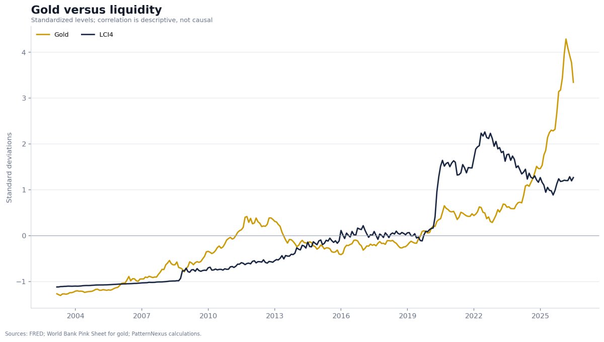
Gold rises from $359 per troy ounce in February 2003 to $4,228 in June 2026, an increase of approximately 1,078%. CPI rises approximately 81% over the same endpoints. The latest twelve-month gold increase in the closed panel is 26.1%. These facts are consistent with gold serving as a long-run monetary hedge, but they do not identify one balance-sheet cause.
The contemporaneous correlation between the monthly change in LCI4 and the monthly log return on gold is −0.005. At a four-month positive asset lag, the correlation is +0.113. At six months it is −0.158. The signs and magnitudes do not support a fixed “liquidity moves first, gold follows” rule.
NASDAQ: discount-rate sensitivity plus an independent earnings engine
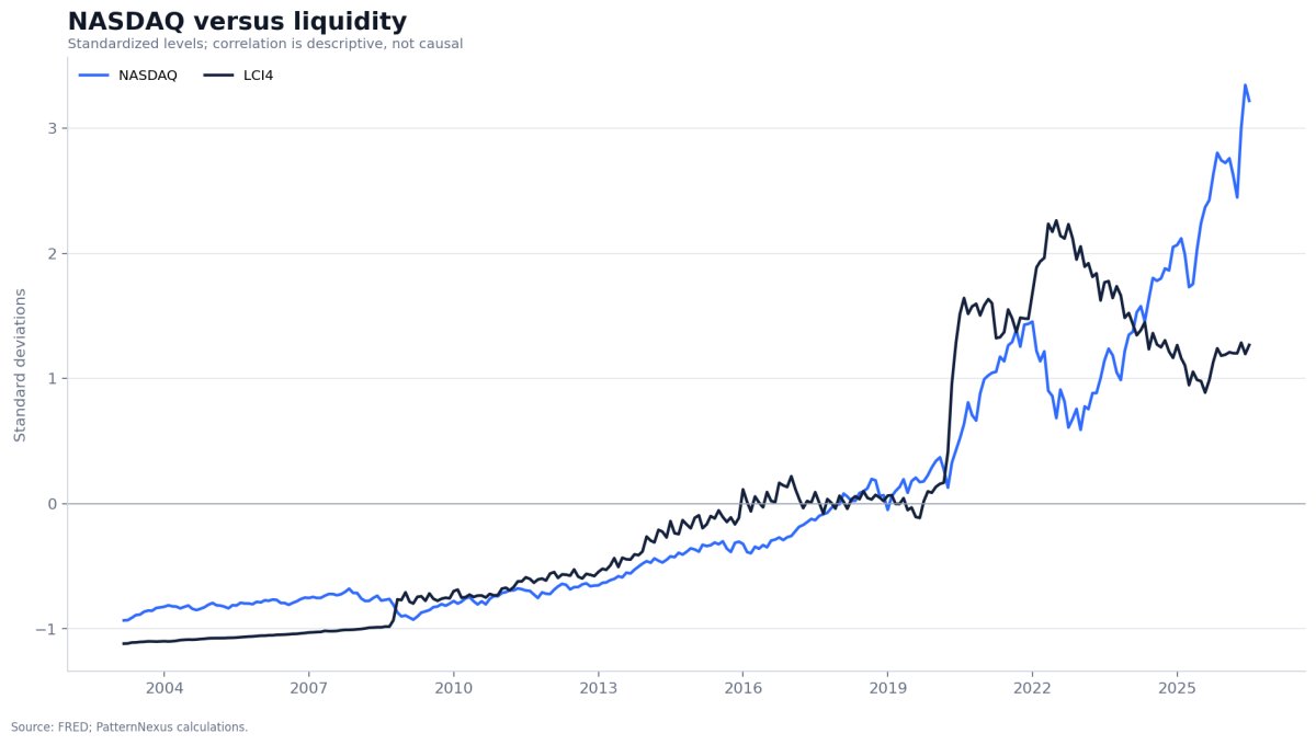
The NASDAQ Composite increases approximately 1,852% from February 2003 through June 2026 and 28.7% over the latest twelve months in the closed panel. Long-duration equities are sensitive to the discount rate applied to future earnings. Liquidity can compress risk premia, ease financing and encourage investors to pay for distant growth. But the index is also a claim on corporate profits, innovation, market structure and competitive advantage.
The monthly-change correlation with LCI4 is −0.107. The largest positive value in the LCI4 lead-lag scan is +0.119 when NASDAQ leads the index by five months. That is compatible with markets anticipating policy or with both variables responding to a third force. It is not evidence that the factor reliably forecasts next month’s equity return.
Housing: the highest level fit and the slowest transmission
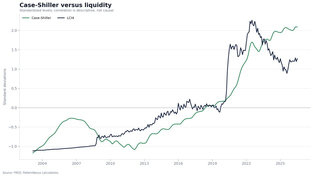
A home is simultaneously a consumption service, a scarce local asset, a leveraged balance-sheet position and the collateral behind a large credit system. National home prices respond to mortgage rates, underwriting, income, demographics, construction, taxes, insurance, local inventory and the financing of the marginal buyer. Liquidity belongs in that system, but no national balance-sheet factor can represent every local market.
Case-Shiller rises 159.2% between the February 2003 and June 2026 panel endpoints. Because the latest raw home-price observation is April and is carried into June, the latest available year-over-year increase is approximately 0.3%. CPI rises 3.5% year over year, rent CPI 2.8% and production-and-nonsupervisory hourly earnings 3.4% over their corresponding latest periods. The home-price level remains high while its rate of appreciation has slowed sharply.
| Asset proxy | Total change, Feb. 2003–Jun. 2026 | LCI4 level correlation | LCI4 monthly-change correlation | CPI level correlation | CPI monthly-change correlation |
|---|---|---|---|---|---|
| Gold | +1,077.7% | 0.701 | −0.005 | 0.879 | 0.159 |
| NASDAQ | +1,852.3% | 0.854 | −0.107 | 0.939 | 0.045 |
| Case-Shiller | +159.2% | 0.875 | 0.053 | 0.922 | 0.225 |
The CPI columns require precise language. The level statistic compares the cumulative CPI index with the asset-price level. The change statistic compares monthly log CPI changes with monthly log asset returns. CPI’s higher figures do not prove that consumer inflation causes the asset moves. They prove that the literal exclusion “not inflation” cannot be justified by raw correlation.
Cross-asset conclusion: LCI4 preserves a strong visual regime relationship, particularly in levels. It does not explain the full amplitude, timing or valuation of any asset. The later robustness tests determine how much weight the visual comparison deserves.
Gold against the four traditional liquidity inputs
Gold is the cleanest conventional hard asset in the study and the asset most directly connected to monetary confidence. It has no coupon, no earnings stream and no tenant. Its price is therefore highly sensitive to opportunity cost, real yields, currency expectations, reserve policy, geopolitical risk, official-sector purchases, mine supply, investment flows and positioning.
The source repair deserves emphasis. The World Bank monthly average is used for every observation in this reconstruction. That avoids an internal splice, but it means the 2026 charts are not numerically identical to charts built from a daily London fixing. A monthly average dampens within-month extremes and should not be compared with a single-day quote without stating the difference.
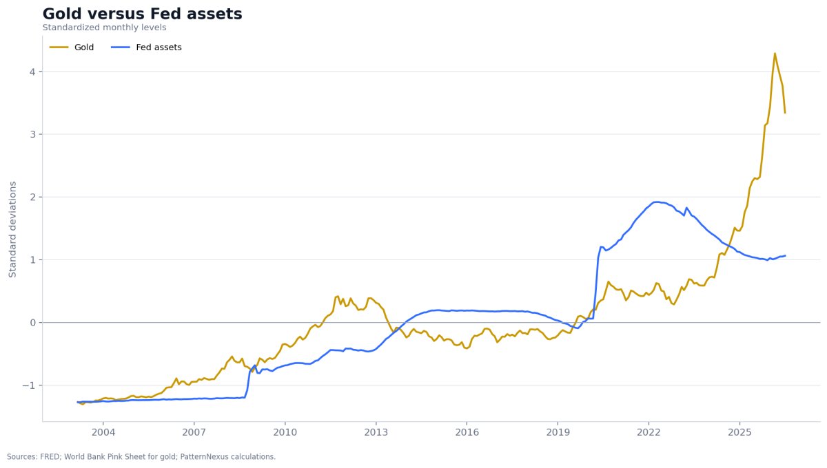
The mechanism is plausible but not one-dimensional. Asset purchases can suppress term premia and reduce the quantity of duration held by the private sector, while gold can benefit when investors question the future purchasing power or fiscal sustainability of nominal claims. During acute funding stress, however, gold can also be sold to raise dollars. The same asset can behave as a hedge in one phase and as a liquid source of cash in another.
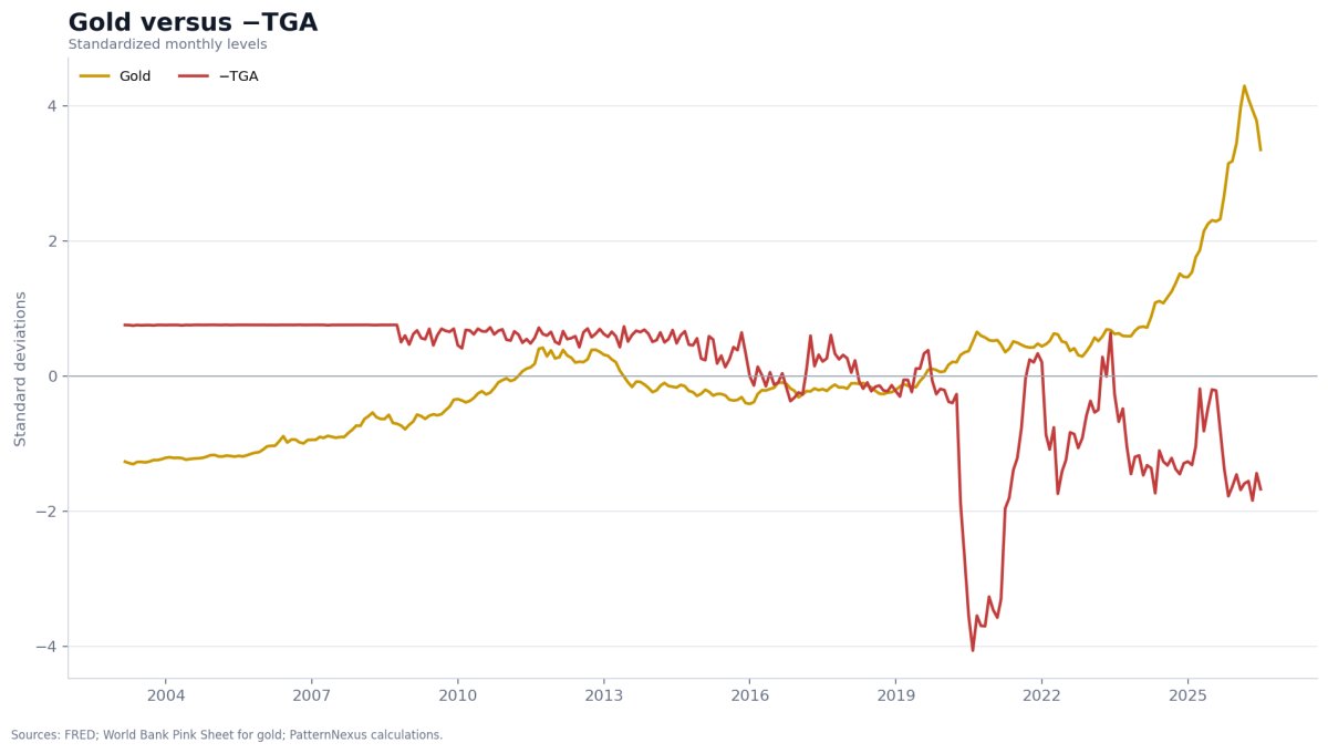
This is a falsification chart for the simple “Treasury spend-down powers gold” narrative. TGA flows can alter reserve and deposit conditions over short horizons, but the full-sample relation is neither consistently positive nor proportional. A durable gold thesis needs information about real yields, fiscal expectations, official-sector demand and the dollar, not just Treasury cash.
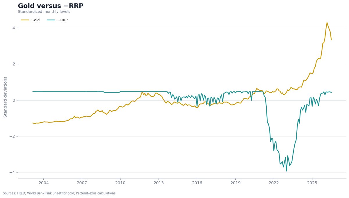
Cash leaving RRP may purchase bills or repo rather than gold. The modest positive change correlation is compatible with some local transmission, but it is far too small to establish a dependable valve from the facility into bullion.
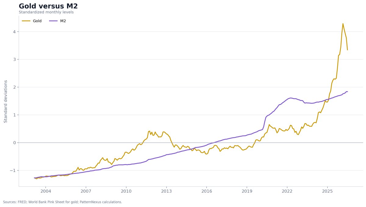
The M2 chart captures the broad monetary denominator argument better than the faster plumbing series. More money-like claims exist relative to a scarce metal across the long sample. Yet the weak change statistic shows why that denominator is a climate, not a calendar. The current gold price has moved far above what a one-factor extrapolation of LCI4 or M2 would imply.
Gold conclusion: liquidity and money are foundational parts of gold’s regime. They do not replace real yields, reserve diversification, geopolitics, fiscal credibility or positioning. Gold is a monetary asset with multiple monetary drivers, not the output cell of one liquidity equation.
NASDAQ against the four traditional liquidity inputs
The original article called NASDAQ the “purest liquidity expression.” That phrase captures the index’s sensitivity to discount rates, funding conditions and risk appetite, but it understates the cash-flow side of the valuation. Technology companies can generate real earnings, network effects and productivity gains. A liquidity regime influences the multiple paid for those earnings; it does not create the earnings by itself.
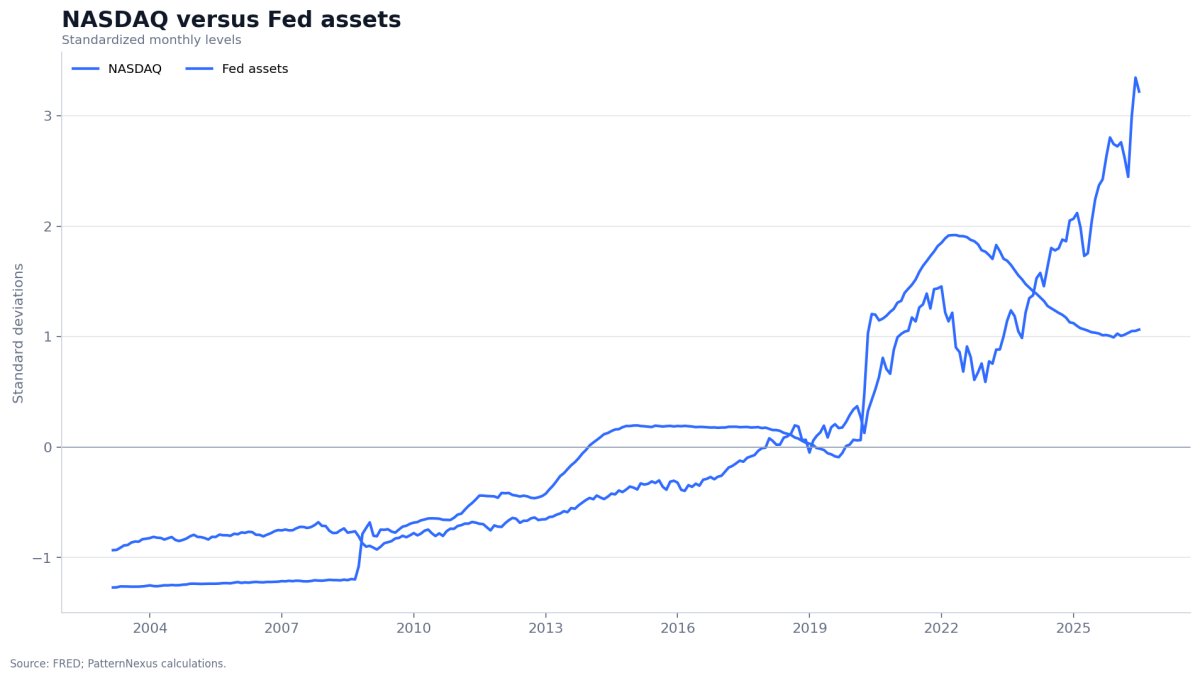
A lower discount rate increases the present value of distant expected cash flows, all else equal. Easier financial conditions can also support venture formation, buybacks, leverage, market depth and investor willingness to hold convex growth exposure. But “all else equal” is rarely true. The artificial-intelligence infrastructure cycle, index concentration and earnings revisions are now central to NASDAQ’s path.
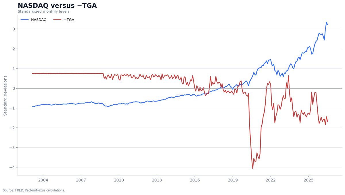
A high TGA can create a marginal drain, but it cannot tell an investor whether earnings expectations are accelerating, whether real yields are falling, whether market breadth is healthy or whether a concentrated group of companies is carrying the index. TGA belongs in the operating dashboard, not in place of an equity model.
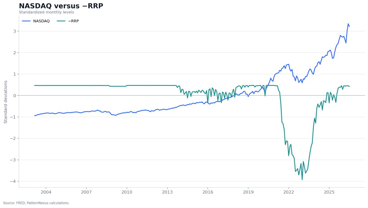
The difference between the negative level statistic and positive change statistic is instructive. The facility’s pandemic-era scale creates an unusual historical shape, while local declines may still ease the safe-asset and funding complex. This is exactly the type of series where a full-sample level correlation can obscure the operational mechanism.
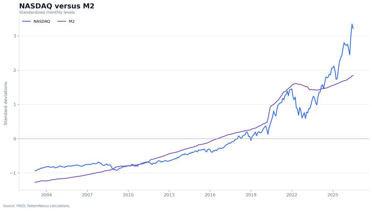
M2 and NASDAQ share a powerful nominal and financial trend, especially through the pandemic expansion. But an investor who traded every monthly M2 change as an equity signal would confront a relationship too weak and unstable for standalone use. The better application is to ask whether broad money reinforces or fights the earnings, valuation and real-rate regime.
NASDAQ conclusion: liquidity affects the price paid for duration and the system’s capacity to finance risk. Earnings, competitive advantage and capital investment determine whether the underlying companies justify that price.
The Colombo comparison was incomplete; liquidity does not make it disappear
The viral housing chart asked a legitimate question: how far can home prices rise relative to CPI, rent and wages before affordability and cash-flow constraints matter? The original Pattern Nexus response correctly added the capital-system layer but went too far when it treated the consumer variables as almost irrelevant.
Housing cannot be analyzed as only a consumer good or only a financial asset. Owner-occupied housing delivers shelter services, secures debt, receives tax treatment, competes with rental housing, depends on local land and construction, and trades through a market whose existing owners often carry long-duration fixed-rate mortgages. Those features create unusually slow and state-dependent transmission.
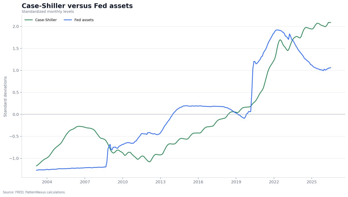
Low rates, income support, deposit creation, mortgage forbearance, household formation and a shift in housing demand all interacted during the pandemic. WALCL is part of that system, but it cannot isolate which channel drove the marginal home purchase.
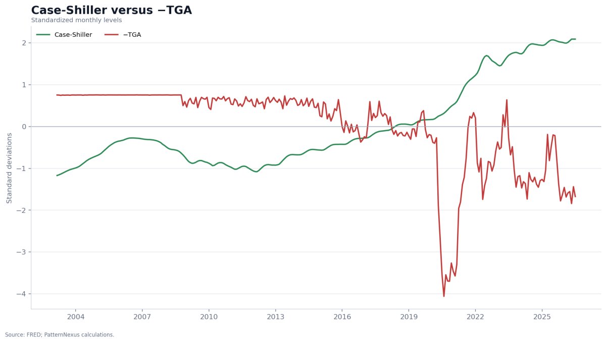
A TGA drawdown can support deposits while the mortgage rate rises, underwriting tightens or listed inventory disappears. Those forces can point in different directions. The monthly national index also averages a housing system with enormous geographic dispersion.
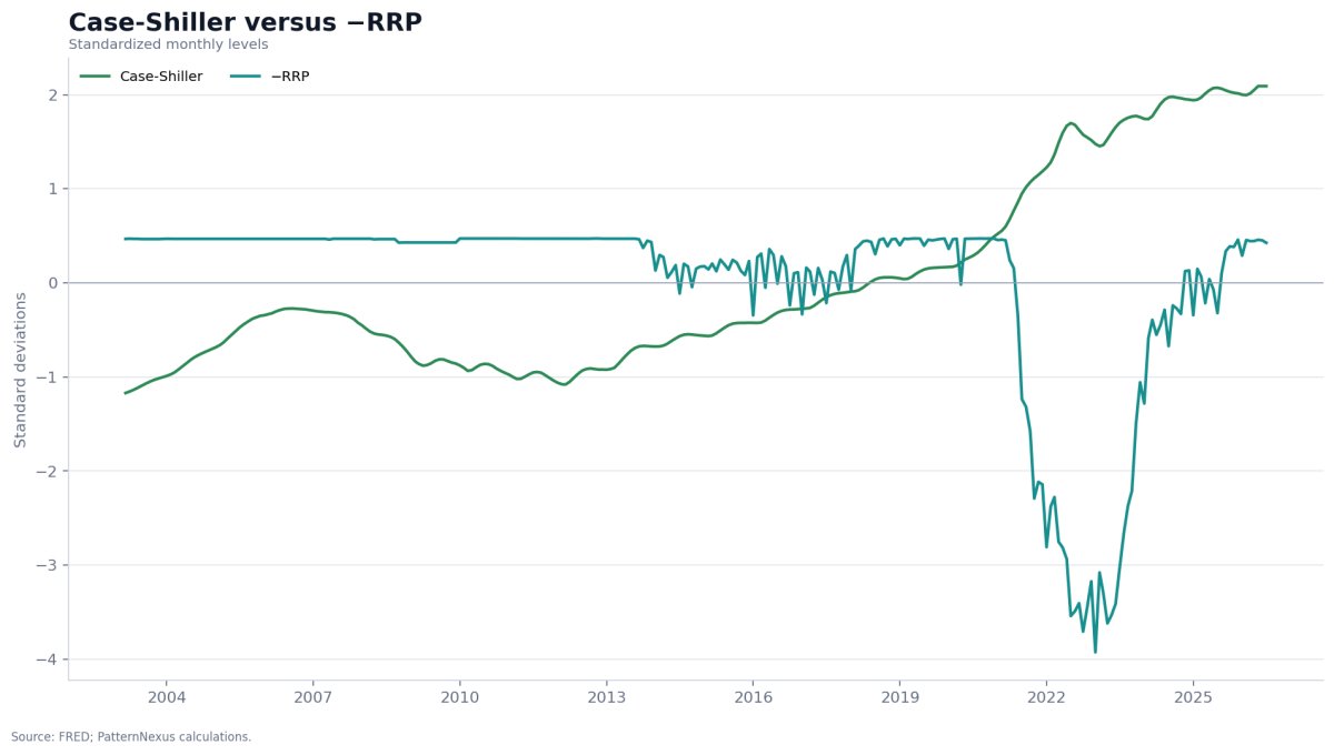
The negative change statistic is a direct warning against treating the RRP drain as a universal housing injection. Money-fund reallocations affect the front end of the financial system first; their path into mortgage credit and local home bids is indirect.
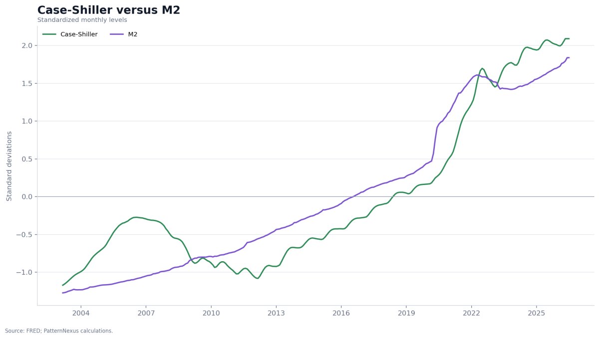
M2 is the most plausible of the four components for describing the long monetary backdrop faced by households. Yet mortgage credit is priced through interest rates, income qualification, lending standards and the housing stock. A large deposit base does not guarantee that a prospective buyer can qualify for the monthly payment on the marginal home.
The affordability chart describes a real divergence
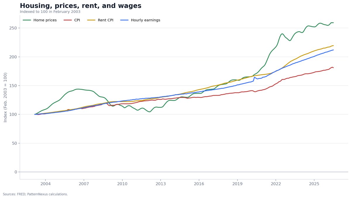
From February 2003 through June 2026, Case-Shiller rises 159.2%, CPI 81.1%, rent CPI 119.4% and production-and-nonsupervisory hourly earnings 111.9%. A household entering the market without existing housing equity faces a larger asset-price increase than the growth in the wage measure. An incumbent homeowner with a low fixed mortgage experiences a different reality because the market value rises while the financing cost remains locked.
This is why “not a bubble because liquidity” is no more complete than “a bubble because prices outran wages.” Liquidity can explain how a valuation gap opens and persists. It cannot guarantee that the gap is affordable, socially stable or immune to a future adjustment.
Adding liquidity changes the story without erasing consumer constraints
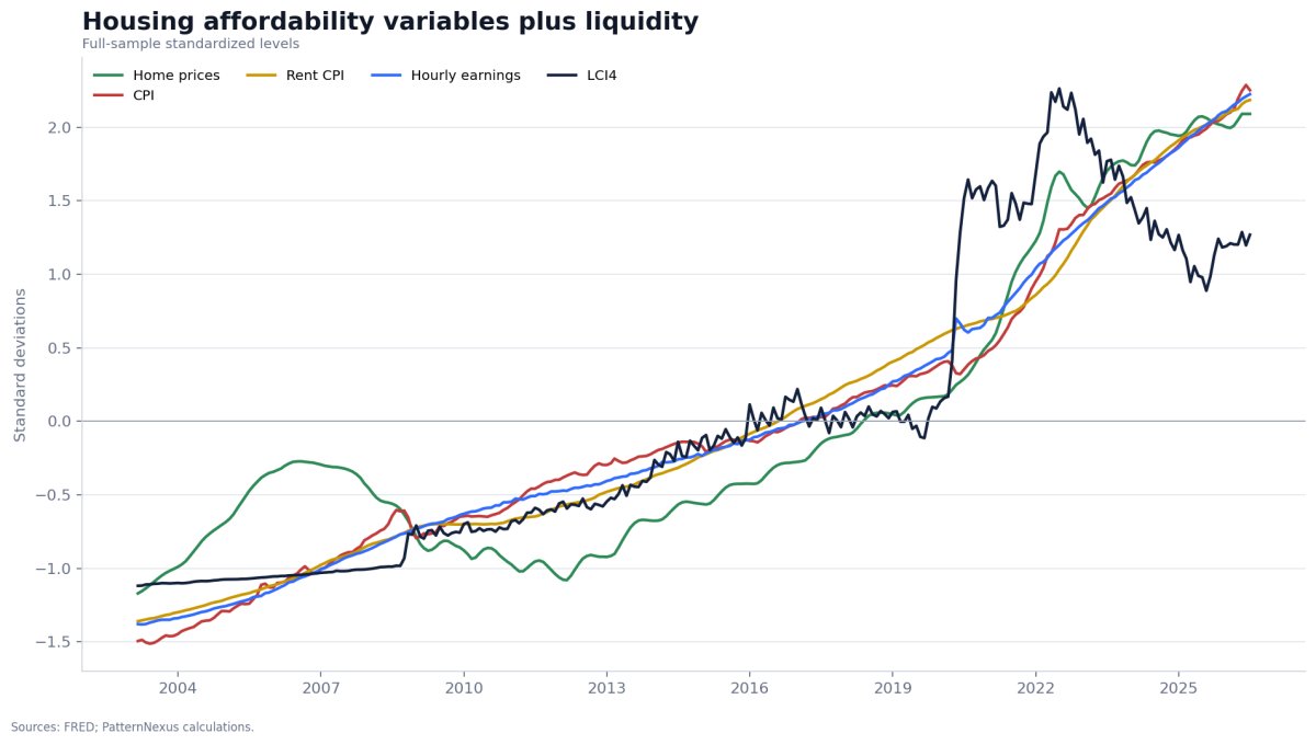
The chart supports a two-system interpretation. Capitalization conditions can move quickly. Contractual rents, wages, construction, housing turnover and consumer prices adjust with longer and uneven lags. But the raw statistics do not establish that the capital system is separate from the consumer economy. The monthly mortgage payment links interest rates and asset prices directly to household income. Construction wages and materials affect replacement cost. Rent and ownership compete at the margin.
CPI’s 0.922 level correlation with Case-Shiller exceeds LCI4’s 0.875. The monthly log-change correlation is 0.225 for CPI versus 0.053 for LCI4. Both are descriptive. The correct conclusion is not that CPI governs housing; it is that the evidence cannot support excluding CPI or affordability variables from the model.
Housing conclusion: liquidity can reprice financing capacity and collateral quickly, while supply, contracts and household behavior slow the adjustment. That explains persistence. It does not eliminate valuation risk or the lived burden on buyers without existing equity.
The level charts are the opening evidence, not the final answer
The original reconstruction derived much of its force from standardized levels. That is understandable: when LCI4, gold, NASDAQ and housing are placed on a common scale, their long regimes often appear to move together. The pictures are informative because they reveal common historical structure. The mistake is to treat that structure as sufficient identification.
Standardization subtracts a series mean and divides by its standard deviation. It changes the units; it does not remove a deterministic or stochastic trend. If two nominal quantities rise over two decades, they can have a high level correlation even when their monthly innovations are unrelated. The same issue applies to CPI, M2, wages and most nominal asset-price indices.
| Asset proxy | LCI4 level | LCI4 monthly change | CPI level | CPI monthly change |
|---|---|---|---|---|
| Gold | 0.701 | −0.005 | 0.879 | 0.159 |
| NASDAQ | 0.854 | −0.107 | 0.939 | 0.045 |
| Case-Shiller | 0.875 | 0.053 | 0.922 | 0.225 |
The comparison does not establish that CPI “wins.” CPI is also a trending nominal index and can stand in for common time, the cumulative change in the dollar price level, wage and revenue growth, policy response and broad money expansion. The result establishes a narrower and more important point: the raw level correlations cannot prove the literal phrase “liquidity, not inflation.”
The monthly-change test asks a more demanding question. Does an increase in the liquidity factor during one month coincide with an asset return or a home-price change during the same month? For gold, the answer is effectively no across the full sample. For NASDAQ, the contemporaneous sign is negative. For housing, it is positive but small. Those results do not erase slower transmission or common regimes. They do reject the idea of a stable one-month multiplier.
Rolling windows reveal the changing relationship
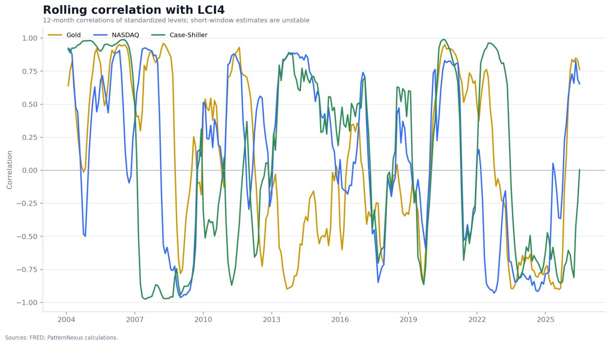
The rolling chart is one of the most consequential tests in the reconstruction. A universal short-horizon driver should produce relationships that remain directionally stable. Instead, all three series travel through positive, negative and near-zero windows. The local alignment depends on the policy regime, the asset’s own cycle and the start and end points inside each window.
At the current endpoint, gold and NASDAQ retain positive twelve-month level alignment with LCI4. Housing does not. The near-zero housing reading does not mean liquidity has no effect on housing. It means the latest twelve observations do not describe home-price levels as a close linear function of LCI4 levels.
The 36-month change correlations provide an even stricter current reading: +0.175 for gold, +0.007 for NASDAQ and −0.062 for housing at June 2026. Over a three-year window, changes in the continuity factor contain only modest contemporaneous information about gold returns and almost none about NASDAQ or national home-price changes.
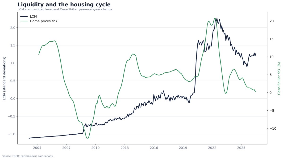
Housing is the most plausible candidate for a slow response because transactions, appraisals, mortgage approvals and index publication all take time. The chart shows broad episodes in which liquidity and home-price growth move through related cycles. It also shows why no fixed lag should be asserted. Credit standards, mortgage rates, construction, household formation and the stock of homes for sale change the transmission in each episode.
Why a higher level correlation can coexist with a weak change correlation
Suppose the financial system moves from a low-liquidity decade into a high-liquidity decade. Asset valuations may also move to a higher regime. Once both have arrived there, month-to-month changes can be dominated by earnings, policy surprises, positioning, mortgage rates or supply. The level chart preserves the regime shift; the change statistic shows that marginal timing is noisy.
That distinction is practical. A regime factor can influence the range of sustainable valuations, the ease of refinancing and the probability of stress without predicting the sign of every monthly return. Investors often need both kinds of information: a slow strategic prior and a faster confirmation signal.
Robustness verdict: the level evidence supports liquidity as a long-horizon regime lens. The change and rolling evidence rejects a mechanical, invariant or stand-alone timing rule. Both statements are required for an accurate conclusion.
A lag scan can locate patterns; it cannot manufacture causality
The original article argued that liquidity moved first and hard assets followed. That is a testable proposition, but it requires a precise definition. This reconstruction correlates monthly changes in each liquidity index with monthly asset changes at lags from −12 to +12 months. A positive lag means the liquidity change occurs first and the asset change is shifted later. A negative lag means the asset leads the index.
| Model | Asset | Largest positive correlation in scan | Lag | What the selected lag says |
|---|---|---|---|---|
| LCI4 | Gold | 0.113 | +4 months | Small positive liquidity-leads result |
| LCI4 | NASDAQ | 0.119 | −5 months | NASDAQ leads LCI4 in the best positive pairing |
| LCI4 | Case-Shiller | 0.125 | +12 months | Small, slow housing response |
| LCI5 | Gold | 0.168 | −8 months | Gold leads the five-input factor |
| LCI5 | NASDAQ | 0.191 | −5 months | NASDAQ again leads the fitted factor |
| LCI5 | Case-Shiller | 0.252 | +12 months | Strongest positive liquidity-leads result, still modest |
The housing result is directionally consistent with a slow financing channel: the best positive relationship occurs one year after the liquidity change in both models. The magnitude improves in LCI5, but 0.252 is still far below a deterministic relationship. For NASDAQ, the best positive result runs in the opposite temporal direction. A forward-looking equity market may anticipate policy, or both policy and equities may respond to information not included in the model.
Gold is unstable across specifications. LCI4’s selected positive result places gold four months after liquidity; LCI5’s places gold eight months before the factor. That change is a warning that the estimated lag is not a deep law. It depends on the input set, sample period and extreme episodes included in the calculation.
The multiple-comparison problem
Each asset-model pair is searched across 25 lags. Selecting the largest positive number after viewing all 25 makes that number look more impressive than a lag chosen in advance. With six asset-model pairs, the exercise inspects 150 correlations. Some local maximum is inevitable even if the underlying relation is weak.
A stronger test would pre-register the lag, fit the model on an earlier period, carry its standardization and loadings forward without revision, and evaluate later returns on untouched data. It would also compare the result with simple baselines and control for real rates, volatility, growth, credit spreads and asset-specific variables. None of that can be replaced by a compelling historical overlay.
Mechanisms still matter
Rejecting causal certainty does not make the plumbing irrelevant. A Fed purchase can change reserves and duration held by the public. Treasury cash operations can change deposits and reserve balances. RRP flows can alter the allocation of money funds across safe assets. M2 can describe the stock of transaction-ready money held by the private sector. Stablecoins can extend settlement reach and on-chain collateral access.
The causal chain, however, contains intervening decisions. Banks choose whether to lend. Dealers choose whether to intermediate. Households choose whether to spend or repay debt. Funds choose which assets to purchase. Issuers choose whether to refinance or invest. Policy expectations move before policy data. An empirical model that omits those choices can describe the environment without proving the final asset-price effect.
Causality boundary: the lag scan supports a plausible slow housing channel and rejects a universal sequence across assets. It should generate hypotheses for out-of-sample testing, not forecasts selected from the best historical lag.
The original cycle remains useful as a map, not as a clock
The original article organized the liquidity story into four recurring phases: build-up, expansion, absorption and contraction. That framework deserves to remain because it forces the reader to ask which balance sheet is moving and where cash is accumulating. The error was presenting the sequence as mechanical, complete and precisely timed.
| Phase | Typical plumbing | Potential asset effect | Main reason the phase can fail |
|---|---|---|---|
| 1 · Build-up | Central-bank assets or broad money begin expanding; Treasury cash may accumulate; funding stress eases unevenly | Financial conditions stabilize before broad risk appetite fully returns | New cash can remain trapped in safe assets, reserves or precautionary balances |
| 2 · Expansion | Multiple channels point easier; credit and collateral capacity improve; risk premia compress | Gold, equities and property can reprice to a higher capitalization regime | Inflation, restrictive rates, valuation or supply shocks can offset the impulse |
| 3 · Absorption | TGA or RRP balances rise, issuance changes collateral, policy support slows or private leverage reaches limits | Asset breadth narrows; the same liquidity stock produces less marginal response | Earnings, scarcity or foreign demand can keep selected assets rising |
| 4 · Contraction | Balance sheets shrink, money growth slows, refinancing costs rise and buffers are depleted | Fragile or highly financed assets become more vulnerable | Policy expectations and private innovation can turn before the measured data |
2003–2007: credit expansion outside the four-input model
The early sample is a reminder that private credit can expand even when the public balance-sheet proxies look uneventful. Mortgage finance, securitization and bank balance sheets mattered enormously before the global financial crisis. LCI4 captures the slow M2 and Fed-balance-sheet backdrop but omits the underwriting deterioration and leverage embedded in housing credit. The period cannot be explained by the four pipes alone.
2008–2012: crisis response and the first modern balance-sheet regime
The global financial crisis produced a dramatic expansion in Federal Reserve assets and a reorganization of collateral and bank reserves. Gold responded strongly through the crisis and sovereign-risk aftermath. Equities fell before recovering. Housing continued to decline because distressed supply, impaired borrowers, foreclosures and damaged credit transmission overwhelmed the new reserve stock. This episode is the clearest demonstration that an easier central-bank balance sheet does not move every asset simultaneously.
2013–2019: normalization, private growth and repeated policy pivots
Federal Reserve asset purchases ended and later balance-sheet runoff began, while M2 continued its slower structural rise. Technology equities compounded through earnings growth, platform economics and falling discount rates. Gold spent years below its prior peak. Housing recovered gradually under tighter supply and repaired household balance sheets. The different paths support a regime interpretation but contradict a single response clock.
2020–2022: synchronized expansion, then offsetting absorption
The pandemic period is the strongest visual support for the original thesis. Federal Reserve assets and M2 surged, fiscal transfers expanded private deposits, risk premia compressed, and gold, equities and housing repriced. The TGA also accumulated cash and ON RRP later grew above $2 trillion, showing that even this apparent textbook phase contained simultaneous injection and absorption.
LCI4 peaks in June 2022 rather than at the first moment of policy expansion. That late peak reflects the full-sample PCA weights and the persistent level of WALCL and M2, not a simple contemporaneous measure of the marginal impulse. Inflation and policy rates had already changed the asset environment by then.
2022–2024: runoff, RRP drainage and asset divergence
Fed assets declined from their peak, M2 contracted for a period, and the TGA remained an offset at various points. At the same time, the enormous ON RRP stock drained toward the market. The combination helped prevent the traditional plumbing story from being uniformly tight. Gold strengthened and technology equities recovered while national housing proved resilient because many owners were locked into low mortgage rates and listed inventory remained constrained.
2025–July 2026: large stocks, fewer buffers and stronger asset-specific forces
M2 and the Fed balance sheet remain historically large, but the LCI4 continuity factor is below its 2022 high. ON RRP is essentially exhausted, which removes both a prior drain and a source of future offset. Stablecoin supply is far larger than in the original sample, while its most recent monthly direction has softened. Gold and NASDAQ have advanced much faster than the current continuity factor. Housing appreciation has slowed toward zero even though the national price level remains high.
This is not a clean phase transition. It is a split regime in which the stock of money-like claims is supportive, the marginal traditional impulse is mixed, and asset-specific engines are dominant. Calling it simply “expansion” or “contraction” would discard more information than it preserves.
Cycle verdict: retain build-up, expansion, absorption and contraction as an operating vocabulary. Diagnose them component by component and allow mixed states; do not infer that all assets must pass through the phases together.
Gold can move first, equities can amplify and housing can persist—but not reliably
The original response hierarchy proposed a compelling sequence: gold responds first to monetary expansion, growth equities amplify the liquidity move, and housing follows slowly because credit and transactions take time. The mechanisms are plausible. The updated data supports pieces of the hierarchy but does not support a fixed ordering.
Gold: the fastest monetary referendum
Gold trades continuously, has no underwriting process and can react immediately to real yields, currency expectations, reserve policy and geopolitical risk. Those features make an early response plausible. Yet the lead-lag results do not produce a stable gold lead or lag across LCI4 and LCI5. Gold’s recent rise far beyond the continuity factor also points to official-sector demand and reserve diversification that the model does not contain.
NASDAQ: the most reflexive capitalization channel
Growth equities combine liquid trading with long-duration cash flows. A lower discount rate or lower risk premium can produce a large present-value change, while rising equity prices can improve financing conditions, employee compensation and acquisition currency. That reflexivity can amplify a liquidity regime. The same index can also lead policy expectations, and current earnings or technological investment can dominate the macro factor for years.
Housing: the slowest observable price index
Housing requires search, financing, appraisal, closing and later index publication. Existing fixed-rate mortgages slow turnover and limit forced selling. Construction responds over long horizons, and supply constraints differ by location. The positive twelve-month lag result is consistent with slow transmission, but affordability and mortgage rates can interrupt or reverse it.
| Asset | Why liquidity can matter | Why the hierarchy can break | Required confirmation |
|---|---|---|---|
| Gold | Real-rate sensitivity, reserve demand, currency confidence, liquid global market | Central-bank purchases, geopolitics, positioning and mine supply can dominate | Real yields, dollar direction, ETF flows and official-sector demand |
| NASDAQ | Long-duration valuation, financing conditions and risk-premium compression | Earnings, concentration, regulation and capital spending can dominate | Earnings revisions, breadth, credit spreads and valuation |
| Housing | Mortgage credit, collateral values, deposit stock and slow supply | Rates, underwriting, income, insurance, taxes and local inventory bind | Mortgage payments, transactions, listings, delinquencies and construction |
The hierarchy is therefore best treated as a mechanism checklist rather than a trading sequence. If gold moves without improving liquidity, inspect real yields and reserve demand. If NASDAQ rises while LCI4 falls, inspect earnings and concentration. If housing remains high while transactions collapse, inspect mortgage lock-in and supply. Divergence is diagnostic information, not a reason to force the asset back into the model.
Hierarchy verdict: the assets have different transmission speeds and amplifiers, but the data does not establish an invariant gold-then-equities-then-housing sequence. Confirmation must be asset-specific.
A fifth liquidity rail is now too large to ignore—and too easy to misclassify
USD stablecoins are tokenized dollar claims that can settle continuously across public blockchains, exchanges, trading venues and increasingly institutional infrastructure. Their macro importance comes less from the label “crypto” than from the settlement rail: a dollar-like instrument can move globally, programmatically and outside traditional banking hours.
That does not mean each token issued is a newly created net dollar. If an issuer receives a bank deposit and purchases a Treasury bill, the transaction may transform an existing claim rather than expand aggregate private-sector wealth. The effect depends on the reserve asset, the seller, the banking flow, the token’s velocity, its use as collateral and whether it enables access that did not previously exist.
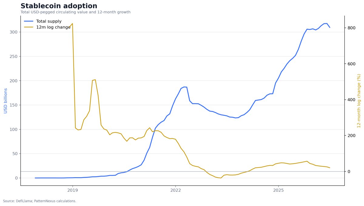
The historical total is sampled at month end from DefiLlama’s USD-pegged series.[14] The current number is a reproducible extraction, not a claim that the live web dashboard will display the same value after later revisions or methodology changes.
The adoption proxy is defined as the z-score of the natural log of total USD-pegged circulating value. Logging compresses a market that grew by orders of magnitude and makes proportional changes more comparable. Standardization then places the logged series on the same numerical scale as the traditional inputs. No value is assigned before November 2017; the unavailable history remains blank.
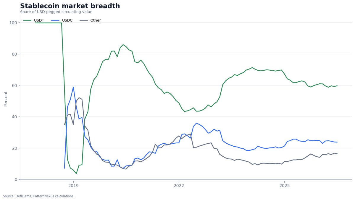
Concentration is not a footnote. A category total can appear broad while reserve, operational, regulatory and redemption risk remains concentrated. USDT and USDC also differ in issuer structure, reserve management, jurisdictional exposure and distribution. A later model should separate fiat-backed, crypto-collateralized and yield-bearing products rather than assume equal liquidity quality.
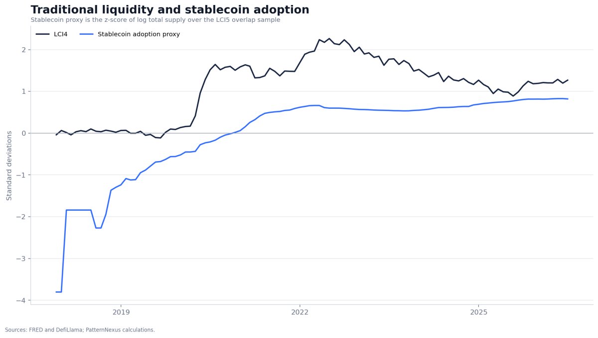
On the shared November 2017–June 2026 sample, log stablecoin levels correlate 0.697 with log gold, 0.815 with log NASDAQ and 0.853 with log Case-Shiller. Monthly-change correlations fall to +0.152, +0.072 and −0.041. Once again, the adoption level shares a strong secular rise with asset prices while short-run changes contain far less common information.
LCI5: a controlled extension, not a rewrite of LCI4
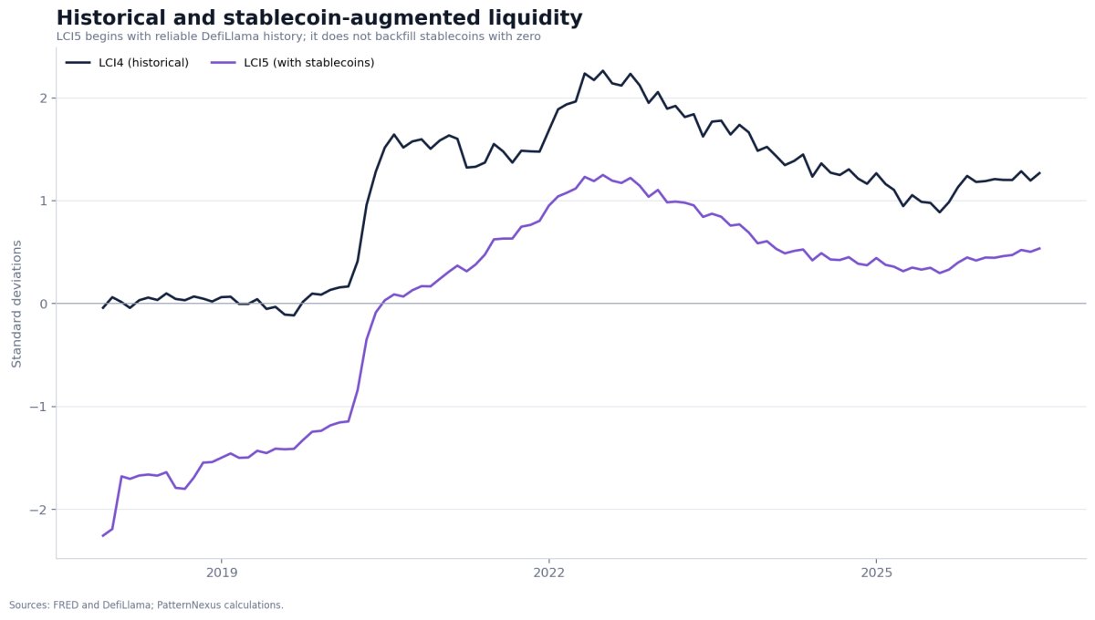
LCI5 adds the standardized log stablecoin-adoption input and is fitted only where all five inputs exist. It begins in November 2017, contains 104 closed monthly observations through June 2026 and excludes the partial July row from estimation. It does not backfill early stablecoin history and does not replace LCI4.
The first LCI5 component explains 64.00% of standardized input variance and correlates 0.861 with its equal-weight sign anchor. Its loadings are +0.536 for WALCL, −0.202 for inverted TGA, −0.369 for inverted RRP, +0.529 for M2 and +0.506 for stablecoin adoption. The traditional sign contradiction remains in reduced form, while stablecoin adoption receives a large positive loading.
| Asset proxy | LCI4 level shared era |
LCI5 level shared era |
LCI4 change shared era |
LCI5 change shared era |
|---|---|---|---|---|
| Gold | 0.270 | 0.432 | 0.090 | 0.120 |
| NASDAQ | 0.440 | 0.614 | −0.126 | −0.015 |
| Case-Shiller | 0.673 | 0.815 | 0.121 | 0.167 |
LCI5 improves all three level correlations inside the shared era. It also raises the gold and housing change correlations and moves NASDAQ’s negative change correlation close to zero. The result is promising but entirely in-sample. The five-input PCA is re-estimated on a shorter period dominated by pandemic-era shocks, and stablecoin adoption is strongly trending. A better fit can represent new information, sample-specific overfitting or both.
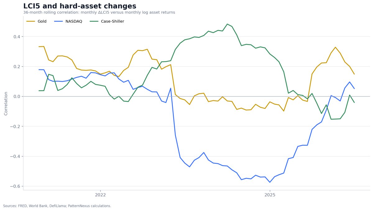
The stablecoin extension improves the description of the post-2017 capitalization regime more clearly than it improves monthly timing. That distinction matters. A structural adoption variable may belong in a long-horizon systems model even if its next-month forecasting power is weak.
Tokenized Treasuries connect the new rail to the old collateral system
The retrieved RWA.xyz snapshot reports $16.197 billion of distributed tokenized U.S. Treasury value across 85 assets and 62,950 holders.[15] These products connect Treasury collateral, stablecoin settlement, fund administration and programmable ownership. They also create potential double counting: a stablecoin issuer may hold Treasury securities while a separate tokenized Treasury represents a direct fund interest. Both relate to the same underlying government debt but serve different holders and functions.
Tokenized Treasuries are not inserted into LCI5 because the reconstruction does not have a comparable open monthly series for the entire five-input window. The current snapshot is preserved as context instead of being converted into an invented history.
A future digital-liquidity module should separate circulating stablecoin value, transfer and settlement volume, issuer reserve composition, exchange leverage, tokenized Treasury ownership outside stablecoin reserves, and cross-chain duplication. Those are different stocks and flows. Adding them together would count wrappers rather than measure balance-sheet capacity.
The current stablecoin signal is not simply “up”
The July snapshot remains 14.8% above the year-earlier level in log-growth terms, which confirms a large ongoing adoption trend. But total supply falls from $317.6 billion in May to $309.5 billion in June and $306.8 billion in the partial July observation. USDT and USDC both soften at the latest endpoint. The annual stock is expanding; the recent marginal impulse is contracting.
That split mirrors the broader dashboard. A large installed base can support market depth and settlement without delivering a fresh monthly acceleration. Readers should distinguish stock from flow, adoption from leverage and dollar tokenization from net money creation.
Stablecoin verdict: tokenized dollars are now a material liquidity rail and belong in the monitored architecture. The available history supports a stablecoin-era extension, but not the claim that stablecoin supply is an independent causal return signal.
The liquidity stock is large; the marginal impulse is mixed
The original article anticipated a forced liquidity expansion in 2026. The current evidence does not justify the word “forced,” and it does not show one clean directional signal. It shows a system with historically large stocks of central-bank assets, broad money and tokenized dollars; an almost exhausted reverse-repo facility; a still-elevated Treasury cash balance; uneven publication dates; and two valid four-input summaries that disagree at the margin.
| Channel | Latest available observation | Current reading | What it means |
|---|---|---|---|
| Federal Reserve assets | July 22 Wednesday level | $6.747T | Historically large balance sheet, below the post-pandemic peak |
| Treasury General Account | Week average ending July 22 | $829.6B | Large Treasury cash stock; future direction depends on receipts, issuance and spending |
| ON RRP | July 24 daily amount | $0.675B | The prior cash absorber is almost empty; little additional drain remains to reverse |
| M2 | May monthly release | $23.052T | High broad-money stock, but stale relative to the July market date |
| USD stablecoins | July 26 extraction | $306.8B | Large and up over twelve months, but down from the May and June endpoints |
| LCI4-PCA | June closed / July live | 1.268 / 1.197 | Above-average continuity level with a negative latest move |
| Equal-weight LCI4 audit | June closed / July live | 0.414 / 0.485 | Conceptually directed inputs show a positive latest move |
| LCI5-PCA | June closed / July live | 0.536 / 0.506 | Positive stablecoin-era level with mild latest softening |
Why the two LCI4 readings disagree
Between the June closed row and the July live row, the TGA falls from $918.7 billion to $829.6 billion and ON RRP falls from $26.9 billion to $0.675 billion. Under the pre-PCA economic signs, both moves are easier. WALCL also rises modestly, while M2 is unchanged because May is still the latest published value. The equal-weight audit therefore rises.
The historical PCA factor assigns negative weights to the already-inverted TGA and RRP inputs. Those same July moves pull LCI4-PCA lower. Reporting only the PCA line would convert the covariance structure into an economic conclusion that its own inputs do not support. Reporting only the equal-weight line would break continuity with the original method. The appropriate dashboard displays both and identifies the source of the divergence.
A practical four-regime framework
| Liquidity level | Liquidity direction | Operating interpretation | Confirmation required |
|---|---|---|---|
| High | Rising | Broad financing tailwind with improving impulse | Falling real yields, stronger breadth, easier credit and asset trend |
| High | Falling | Supportive stock but decelerating impulse | Earnings, scarcity or demand must carry more of the move |
| Low | Rising | Early repair, policy turn or buffer release | Funding markets, credit spreads and price confirmation |
| Low | Falling | Fragile refinancing and collateral regime | Stress indicators, defensive balance sheets and policy response |
LCI4-PCA places the system closest to high but falling. The equal-weight audit reads above average and rising in the partial July row. LCI5 reads positive but mildly falling. The disagreement is itself the signal: the regime is not broad-based enough to reduce to one arrow.
Asset conditions are stronger than the composite alone would imply
Gold closes June at a World Bank monthly average of $4,228 per ounce and is up 26.1% over twelve months. NASDAQ closes July 24 at 24,975.82 and is up 28.7% over the latest twelve months in the closed panel. National home prices are nearly flat year over year at the latest April observation, even though the index level remains historically high. The cross-asset dispersion is incompatible with the claim that one liquidity factor sets every asset’s current direction.
Gold’s independent drivers include reserve diversification, official-sector demand, real yields and geopolitical risk. NASDAQ’s include earnings, market concentration and artificial-intelligence investment. Housing’s include mortgage rates, insurance, taxes, household income, construction and the scarcity created by mortgage lock-in. Liquidity modifies those forces; it does not replace them.
What could change the dashboard next
- A sustained TGA drawdown could return cash to the private system, but the effect would depend on the issuance and spending path.
- Renewed Fed balance-sheet expansion would strengthen the traditional stock signal, especially if accompanied by easier real rates and credit.
- Faster M2 growth would reinforce the slow monetary backdrop once the lagged monthly series confirms it.
- Stablecoin reacceleration would strengthen the digital-dollar adoption impulse, particularly if transaction volume and market breadth rise with supply.
- Higher Treasury cash or tighter collateral conditions could offset supportive money stocks.
- Asset-specific deterioration—weaker earnings, wider credit spreads, falling gold demand or rising housing inventory—could overwhelm a supportive liquidity level.
July judgment: the system holds a large liquidity stock but does not deliver a unanimous positive marginal impulse. The current regime rewards component-level analysis and asset confirmation more than confidence in a single composite.
The same plumbing creates different decisions for different readers
A premium macro framework should not stop at a chart interpretation. The stakeholders exposed to liquidity are not interchangeable. An investor chooses risk and time horizon. A homeowner carries a leveraged consumption asset. A corporate treasurer manages cash and refinancing. A policymaker weighs market functioning against inflation and distribution. A stablecoin issuer transforms reserve assets into a settlement claim. The relevant signal and the cost of being wrong differ in each case.
Long-horizon investors and asset allocators
Use the liquidity level as a strategic prior, not a price target. A high stock of money-like claims can support higher nominal asset valuations and reduce the probability that every cyclical slowdown becomes a funding crisis. A falling impulse can still narrow market breadth, expose valuation risk and increase dependence on asset-specific fundamentals.
For gold, pair the dashboard with real yields, dollar direction and official-sector demand. For technology equities, pair it with earnings revisions, free cash flow, concentration and credit spreads. For property, pair it with mortgage payments, inventory, transaction volume and local labor income. The model is most valuable when it identifies which part of an investment case is monetary and which part is not.
Traders and risk managers
The weak monthly-change correlations argue against direct signal execution. A one-month LCI change should not automatically create a long or short position. It can instead influence risk limits, expected volatility and the degree of confirmation required from price, breadth, funding markets and asset-specific catalysts.
The live row must be treated with particular caution. July combines observations from April through July and carries older monthly values forward. A market can move on a new policy expectation before the input series is published. The relevant trading question is often the surprise relative to expectation, not the absolute level later recorded in the database.
Homeowners, prospective buyers and renters
Liquidity explains why home prices can remain high even when affordability looks extreme. It does not reduce the monthly payment. Buyers must still evaluate mortgage rate, down payment, taxes, insurance, maintenance, income stability and the local supply-demand balance. National Case-Shiller is not a valuation model for a specific property.
Existing owners with low fixed-rate mortgages have embedded financing value. That value discourages turnover and can support prices even as transaction volume falls. Renters and first-time buyers do not receive the same benefit, which is why the wealth and access consequences of the housing-liquidity regime can worsen even without a national price decline.
Builders, lenders and housing policymakers
A high national asset-price level can coexist with weak new-project economics when construction finance, labor, materials, insurance and land costs remain high. Lenders should not treat collateral appreciation as a substitute for borrower capacity. Policymakers should distinguish price support from unit production: liquidity can capitalize scarce homes without solving scarcity.
The Colombo comparison remains useful here. The divergence between housing, wages and rent is not disproved by monetary plumbing. It identifies who is being priced out and where the distributional consequences accumulate. A complete housing policy needs supply, credit, tax and income analysis alongside the macro liquidity backdrop.
Corporate treasurers and financial officers
Liquidity conditions influence refinancing windows, investor demand and the opportunity cost of cash. A supportive stock can keep markets open even when the marginal impulse deteriorates. Treasurers should monitor the maturity schedule, floating-rate exposure, covenant headroom and counterparty concentration rather than assume that a positive composite guarantees inexpensive funding.
Stablecoins and tokenized Treasuries may extend operating hours and settlement choices, but they introduce issuer, custody, smart-contract, legal and redemption risks. Yield on a tokenized claim must be evaluated together with the underlying reserve asset and the route by which cash returns to the firm.
Stablecoin issuers, banks and payment firms
The $306.8 billion category scale makes reserve transparency, redemption design and operational resilience macro-relevant. Issuers are increasingly connected to Treasury demand and short-term funding markets. Banks face both deposit displacement and new distribution opportunities. Payment firms face a rail that can settle continuously but whose legal finality and consumer protections vary by structure and jurisdiction.
Growth in supply should not be confused with broad user adoption. Market share, active addresses, transfer volume, settlement value, reserve composition and concentration answer different questions. A durable market requires evidence that scale is not dependent on a small set of issuers, exchanges or leverage loops.
Policymakers and regulators
The model illustrates why policy cannot be read from the policy rate alone. Balance-sheet runoff, Treasury cash management, bill supply, RRP usage, bank deposits and tokenized-dollar growth can offset or reinforce one another. Financial conditions may remain easy in selected assets while consumer credit is restrictive.
Stablecoin regulation can affect Treasury demand, deposit competition, payment innovation and global dollar access at the same time. The objective should be to make reserves, redemption priority, bankruptcy treatment and operational responsibilities legible without pretending that every tokenized dollar has the same risk or economic function.
Researchers, journalists and public readers
The most important discipline is to name the transformation. “CPI” can mean the price-index level or the inflation rate. “Liquidity” can mean a stock, a change, a balance-sheet identity or a fitted factor. “Latest” can refer to different observation months. A chart that does not state these distinctions can be visually correct and analytically misleading.
Readers should ask for the sample, units, frequency, revision policy, missing-data rule, transformation, fitted weights and comparison statistic. The downloadable package is designed so those questions can be answered without reverse-engineering the article.
Real-people translation: abundant system liquidity can raise the market price of assets without making them affordable from current income. That difference benefits existing asset owners, challenges new entrants and makes the distribution of collateral as important as the quantity of money.
How to rebuild the framework without hidden judgment calls
The complete data package is intended to make the article reproducible rather than merely persuasive. A reader can begin with the provider files, repeat the monthly alignment, inspect the transformed inputs and compare the resulting model outputs with the supplied workbook and charts.
Reproduction sequence
- Freeze an extraction cutoff. Record the retrieval timestamp and preserve the raw provider file before a public dashboard or economic series is revised.
- Separate closed and live periods. Fit the historical model only through the latest fully closed monthly bucket. Keep the partial month outside the estimated parameters.
- Map every series to month end. Use the last available observation associated with each month, then carry lower-frequency values forward only after the first valid observation.
- Apply the economic directions. Keep WALCL and M2 positive; multiply TGA and RRP by −1 before standardization. Do not add a pre-history to a series that did not exist.
- Standardize on the declared sample. Use the full closed-sample mean and population standard deviation for the continuity reconstruction. Store those parameters so the live row can be projected without refitting.
- Estimate PCA1 and anchor its global sign. Compare the fitted component with the equal-weight mean of the directed inputs. Flip the entire component only if that correlation is negative.
- Publish the loadings. Do not assume that the global sign anchor forces each loading into the intended economic direction.
- Calculate both levels and changes. Use standardized levels for regime charts and log differences for monthly change correlations where values are positive.
- Run rolling and lagged tests. Treat selected lag maxima as exploratory unless the lag and evaluation period were specified before viewing the results.
- Reproduce LCI5 on its own overlap. Add the standardized log stablecoin total only from November 2017 onward and re-estimate all five-input parameters on that shared sample.
- Validate the output. Check sample endpoints, missingness, z-score means, sign-anchor direction, model freshness and the absence of fabricated stablecoin history.
Monthly monitoring sequence
| Release or market | Typical cadence | Dashboard role | Common mistake |
|---|---|---|---|
| WALCL | Weekly, Wednesday level | Central-bank balance-sheet stock | Treating all assets as immediately deployable reserves |
| WTREGEN | Weekly average | Treasury cash drain or release | Ignoring receipts, spending and issuance composition |
| ON RRP | Daily amount | Money-fund safe-asset buffer | Assuming every decline becomes a risky-asset purchase |
| M2 | Monthly | Broad private money stock | Reading a lagged release as a current-month flow |
| Stablecoins | Continuous dashboard | Digital-dollar adoption and settlement stock | Confusing token issuance with net dollar creation |
| Gold and NASDAQ | Market prices | Fast asset confirmation | Comparing a daily close with a monthly average without disclosure |
| Case-Shiller | Monthly with publication lag | Slow national housing confirmation | Calling the carried value a current home-price observation |
The minimum useful dashboard reports the raw latest values, their observation dates, LCI4-PCA, equal-weight LCI4, LCI5, recent direction and asset-specific confirmation. The method should never hide stale inputs behind a single “as of” label.
Reproducibility standard: another analyst should be able to use the stored source files and declared rules to obtain the same closed-sample parameters and identify exactly why a later live dashboard differs.
What would strengthen the thesis—and what would make it fail
A framework becomes more valuable when it states the observations that could prove it wrong. “Liquidity matters” is too broad to falsify because almost any financial event can be placed under the word after the fact. The testable version must specify the inputs, direction, horizon, asset and comparison model before observing the outcome.
Evidence that would strengthen the framework
- Out-of-sample stability. Weights fitted through an earlier date should retain direction and explanatory power in later data without full-sample re-estimation.
- Economically consistent weights. A constrained or regularized composite should outperform the current PCA while preserving the intended signs for TGA and RRP.
- Incremental information. LCI should add explanatory or predictive value after controlling for real rates, the dollar, volatility, credit spreads, earnings, mortgage rates and inflation.
- Cross-country replication. Comparable balance-sheet measures should explain local asset regimes outside the United States after currency and institutional differences are addressed.
- Event-level transmission. Identified policy or Treasury cash shocks should produce measurable changes in funding, collateral, lending or portfolio allocation before the asset response.
- Digital-rail validation. Stablecoin supply, velocity and reserve composition should improve untouched-period results without relying on the same pandemic-era trend used to fit the factor.
Evidence that would weaken or falsify the framework
- Persistent opposite moves. Hard assets repeatedly rising through broad, multi-channel liquidity contraction—or falling through broad expansion—without asset-specific explanations would weaken the regime claim.
- No incremental value. If simple time trends, CPI, real rates or asset-specific fundamentals fully absorb LCI’s contribution, the composite would add description without analytical edge.
- Unstable specifications. If small changes in sample, frequency, standardization or input definition reverse the model’s conclusions, the factor is not robust enough for decision use.
- Loading incoherence. If economically directed inputs continue to receive opposing weights and the composite repeatedly contradicts a transparent equal-weight audit, PCA continuity would lose its interpretive value.
- Failed real-time tracking. If vintage data and fixed historical parameters do not reproduce the relationships visible in revised full-sample data, the apparent signal may be a look-ahead artifact.
- Stablecoin non-incrementality. If LCI5 fails after the fitted period or the improvement disappears after detrending, stablecoin adoption should remain a separate dashboard item rather than an index component.
A research program that can answer the remaining questions
The next version should maintain a real-time vintage archive, estimate rolling and expanding-window models, compare PCA with constrained equal weights and economically specified arithmetic measures, and report confidence intervals around correlations and lag estimates. It should test changes at monthly and quarterly frequencies and separate crisis from non-crisis periods.
Asset-specific equations should include real yields and reserve demand for gold, earnings and valuation for NASDAQ, and mortgage rates, inventory, credit standards and income for housing. A digital module should include stablecoin transfer volume, reserve mix and tokenized Treasury ownership without double counting the same underlying claim.
Falsification rule: the framework earns confidence only when it adds stable, out-of-sample information beyond simpler models. A persuasive historical overlay is not enough.
What the reconstruction can measure—and what it cannot
The original article included limitations, and they are retained here in expanded form. These are not ceremonial disclaimers. Each limitation identifies a specific way the model can mislead a reader or fail in live use.
1. Correlation and PCA do not identify causality
PCA finds a direction of shared variance. Correlation measures linear association. Neither isolates an exogenous policy shock or shows the path from a balance-sheet entry to a marginal asset buyer. Reverse causality and common omitted causes remain possible.
2. Standardized levels remain trending levels
Z-scoring changes scale, not time-series properties. High level correlations can arise because nominal series share common growth, inflation or time trends. The change and rolling analyses reduce this risk but do not solve every stationarity or cointegration question.
3. The full-sample normalization contains look-ahead information
Every historical z-score uses the mean and standard deviation of the completed February 2003–June 2026 sample. PCA loadings are also estimated on the full period. The result is a retrospective reconstruction, not the sequence of readings an investor would have observed in real time.
4. PCA signs conflict with the economic input design
The already-inverted TGA and RRP inputs receive negative LCI4 loadings. The global sign anchor remains positive but correlates only 0.486 with the equal-weight audit. The continuity series is therefore not a clean monotonic measure in which every conceptually easier input raises the score.
5. The proxies have different units, frequencies and mechanisms
WALCL and TGA are reported in millions, RRP and M2 in billions, and their source observations range from daily to monthly. Standardization makes them numerically comparable, not economically interchangeable. A one-standard-deviation change does not represent the same number of dollars or the same transmission.
6. Forward filling aligns dates but does not create information
M2 and Case-Shiller are carried into later period buckets until a new release appears. That permits a complete panel and live projection. It does not make the April housing value or May M2 value a July observation. Revisions can also alter prior periods after the package cutoff.
7. The gold measurement changed across editions
The World Bank monthly average provides a complete, current and auditable source for this reconstruction. It is not identical to a daily London fixing used in an earlier edition. All months in the present article use the World Bank series, so there is no internal splice, but comparisons between article editions include a provider and frequency difference.
8. The model is U.S.-centric
The four traditional inputs describe U.S. dollar and Federal Reserve plumbing. Gold is global, NASDAQ companies earn globally and housing is local. Foreign central banks, offshore dollar credit, exchange rates, sovereign reserve decisions and non-U.S. regulation can be decisive.
9. Important credit and collateral channels are omitted
Bank lending, private credit, dealer balance-sheet capacity, repo haircuts, Treasury issuance maturity, money velocity, fiscal deficits, cross-border dollar funding and lending standards are not direct model inputs. M2 and WALCL cannot stand in for all of them.
10. LCI5 has a short and unusual history
The five-input model contains only 104 closed months beginning in November 2017. That window includes the pandemic, exceptional fiscal and monetary actions, a large RRP cycle and rapid stablecoin adoption. In-sample improvement may not persist in a normal regime.
11. Stablecoin totals combine different instruments
Fiat-backed, crypto-collateralized, algorithmic and yield-bearing tokens can have different reserve quality and redemption behavior. Circulating value does not measure transaction velocity, unique users, leverage or settlement purpose. Dashboard revisions and chain-level duplication can change totals.
12. National housing data hides local markets
Case-Shiller is a national repeat-sales index with publication lag. It does not include every geography or represent the price, condition, tax, insurance burden or financing of a specific home. National resilience can coexist with severe local declines or shortages.
13. The model contains no valuation anchor
Liquidity can support a high multiple without proving that it is justified. Gold has no cash-flow valuation, NASDAQ has earnings and discount-rate inputs, and housing has rent and user-cost relationships. An asset can remain overvalued in an easy regime or undervalued in a tight one.
14. The lag search is exploratory
Choosing the best result from −12 to +12 months after seeing the data introduces selection bias. The lag table is a map of historical associations, not a confidence interval or a pre-registered forecast test.
15. Structural change can break the historical mapping
Payment rails, bank regulation, Treasury issuance, stablecoin law, collateral practices and market composition evolve. A covariance structure estimated across 2003–2026 can become obsolete even if every calculation is correct.
The inflation comparison, stated precisely
The reconstructed evidence does not support literal exclusion. CPI’s level correlations exceed LCI4’s for gold, NASDAQ and housing, and CPI’s contemporaneous change correlations are also higher in this sample. That does not establish consumer inflation as a sole causal driver. It shows that the price level, money, nominal incomes and asset prices share long-run forces and that a one-variable slogan is underidentified.
The more defensible systems conclusion is that liquidity shapes financing capacity, collateral values, discount rates and portfolio substitution, while inflation shapes real returns, policy response, replacement costs and nominal cash flows. Asset-specific supply and earnings determine how those macro conditions become prices.
Limitations verdict: LCI4 and LCI5 are descriptive regime tools. They are not causal structural models, valuation engines or guaranteed trading signals. Their value depends on transparent inputs, complementary evidence and disciplined use.
The thesis survives as architecture, not as absolutism
The original article’s most durable contribution was to move the conversation upstream. A chart comparing home prices with wages and rents can describe the household outcome while missing the balance-sheet system that capitalizes the asset. The same principle applies to gold and long-duration equities. Asset prices are formed where money, collateral, expected cash flows, financing and scarcity meet.
The update preserves that insight and rejects the claim that one reconstructed factor is the “true underlying driver.” LCI4’s long-run correlations are large. Its monthly-change relationships are weak. Its PCA weights conflict with two economic input directions. CPI produces even higher raw level correlations. The hard assets also diverge sharply at the current endpoint. A model that acknowledges those facts is more valuable than one protected by absolute language.
The supercycle chronology, revised
The 2003–2007 credit expansion showed that private leverage can create a powerful asset cycle outside the selected public plumbing measures. The 2008–2012 response showed that central-bank expansion can stabilize finance while housing continues to fall. The 2013–2019 period showed that earnings, falling discount rates and repaired credit can support equities and housing while gold behaves differently. The 2020–2022 episode showed the force of synchronized fiscal, monetary and money-stock expansion. The 2022–2026 period showed that RRP drainage, mortgage lock-in, reserve diversification, artificial-intelligence investment and stablecoin adoption can sustain selected assets even as the continuity factor retreats.
The supercycle is therefore not a single wave in which every hard asset follows a master index. It is an evolving balance-sheet architecture. Public and private credit, Treasury collateral, bank deposits, central-bank reserves and tokenized dollars interact through changing institutions. The structure can remain liquid while the marginal impulse rotates from one channel to another.
The new paradigm is additive
Stablecoins do not replace the Federal Reserve, banks, M2 or Treasury markets. They add programmable distribution and settlement to the dollar system. Tokenized Treasuries do not create a new sovereign asset; they add a new wrapper, ownership record and transfer rail around government debt. The analytical task is to measure which new rails increase reach, turnover and collateral utility without double counting the underlying dollar claim.
That is why LCI5 is maintained as an experimental extension. It captures the shared post-2017 regime better in-sample, but its short history and strong trend prevent a claim of superiority. The next research edge lies in transaction velocity, reserve composition, collateral reuse and real-time settlement—not in adding the largest available digital number to a macro index.
The 2025–2026 implication
The current environment is neither a simple liquidity boom nor a clean contraction. Gold and technology equities are strong, housing appreciation is nearly flat, ON RRP is almost gone, the TGA is high, M2 is large, stablecoin adoption is high but recently softer, and the PCA and equal-weight LCI4 readings disagree. That configuration demands a systems dashboard rather than a forecast slogan.
A renewed, broad liquidity expansion remains possible. It is not inevitable merely because refinancing needs, fiscal deficits or market stress exist. Policy can choose among rates, balance-sheet tools, Treasury cash management, regulation and fiscal measures. Private balance sheets can absorb or amplify the result. The forecast must remain conditional.
Final judgment: the original category correction stands. Liquidity belongs upstream in hard-asset analysis. The absolute exclusion of inflation and the claim of mechanical prediction do not survive the full reconstruction. The investable insight is conditional: track the stock, direction, composition and freshness of liquidity, then require confirmation from the asset itself.
The article and its audit trail travel together
The paid entry includes two analytical deliverables and one publication asset:
- Hard_Assets_Liquidity_Data_Package_2026-07-26.zip — the full reconstruction package with raw files, processed data, model outputs, charts, documentation, source manifest, validation results and checksums.
- Hard_Assets_Liquidity_Update_July_2026.xlsx — the formatted workbook containing the monthly panel, dashboard, PCA loadings, correlations, freshness schedule, checks, sources, methodology and chart data.
- Pattern_Nexus_Hard_Assets_Liquidity_2026_Hero.png — the publication hero image for the entry’s image field; it is not embedded in this body HTML.
Package structure
| Package area | Contents | Purpose |
|---|---|---|
| data/raw | FRED, World Bank, DefiLlama and RWA.xyz source files | Preserve the exact extraction inputs |
| data/processed | Closed and live panels, z-scores, LCI4, LCI5, correlations, rolling tests and lead-lag results | Expose every analytical transformation |
| charts | All 31 chart files used in this article | Allow chart inspection and republication |
| workbook | Formatted analytical review file | Provide a reader-friendly audit surface |
| manifest and checksums | SOURCE_MANIFEST.csv and SHA256SUMS.txt | Identify provenance and verify file integrity |
| article materials | Locked body HTML and publication fields | Keep editorial and analytical outputs synchronized |
Model specification summary
| Model | Inputs | Closed sample | PCA1 variance explained | Defined role |
|---|---|---|---|---|
| LCI4 | WALCL, −TGA, −RRP, M2 | Feb. 2003–Jun. 2026 | 76.47% | Historical continuity factor |
| Equal-weight LCI4 | Mean of the same four directed z-scores | Feb. 2003–Jun. 2026 | Not applicable | Economic-sign audit |
| LCI5 | LCI4 inputs plus log stablecoin adoption | Nov. 2017–Jun. 2026 | 64.00% | Experimental stablecoin-era factor |
The data package is part of the analysis, not an appendix added for appearance. It makes the source vintages, carried values, transformations, model contradictions and validation results inspectable by readers who want more than the narrative.
Questions readers should ask before using the reconstruction
What is the shortest accurate conclusion?
Liquidity is a first-order regime input for gold, long-duration equities and housing, but it is not the only driver, a valuation model or a reliable stand-alone monthly timing signal. Inflation, real rates, earnings, credit and supply remain part of the causal system.
Is the original LCI still preserved?
Yes. LCI4 remains the sign-anchored first principal component of WALCL, inverted TGA, inverted ON RRP and M2. LCI5 is maintained separately so stablecoin adoption does not rewrite the historical definition.
Why does the closed model stop in June when the article is dated July 26?
June is the latest completed monthly bucket used for estimation. July contains current daily and weekly readings but lagged monthly releases. It is projected through fixed June parameters and flagged as live and partial.
Why is April housing carried into June and July?
Case-Shiller is published with a lag. Forward filling keeps the monthly panel aligned, but the observation date remains April. The article never treats the carried value as a newly measured July home price.
Why was gold moved away from the prior Fed-hosted series?
The earlier route no longer provided a reliable current continuation for this update. The World Bank Pink Sheet supplies an auditable monthly average through June 2026. Every gold observation in the present reconstruction uses that provider, so there is no internal splice.
Does a positive LCI mean assets must rise?
No. A positive score means the fitted factor is above its closed-sample mean. Direction, valuation, real yields, earnings, supply, credit and positioning still determine the asset outcome. The weak and unstable change correlations demonstrate the limitation.
Why are TGA and RRP inverted before PCA?
The conceptual model treats higher Treasury cash and higher reverse-repo balances as money parked away from broader private circulation. Multiplying them by −1 places an easier movement in the positive direction before standardization.
Why can inverted TGA and RRP still receive negative PCA loadings?
PCA is unconstrained. It selects the covariance direction that explains the most variance, not the direction specified by the economic story. The global sign anchor can flip the whole component but cannot force each loading to be positive.
Which LCI4 reading should be trusted in July: PCA or equal weight?
They answer different questions. PCA preserves continuity with the historical covariance factor and falls in the partial July row. Equal weight preserves the intended economic direction of all four inputs and rises. The disagreement should be reported, not resolved by hiding one series.
Why not use Fed assets minus TGA minus RRP as “net liquidity”?
That arithmetic monitor is useful but incomplete. The series use different units and frequencies, M2 is absent, and the economic effect depends on counterparties and collateral. The present package allows readers to construct that alternative while keeping the published models explicit.
Does stablecoin issuance create new money?
Not automatically. It can transform a bank deposit or Treasury-backed claim into a tokenized liability. It can still change settlement reach, velocity, market access and collateral use, which is why adoption matters even when net dollar wealth does not increase.
Why use the log of stablecoin supply?
The category grew by orders of magnitude. The natural log reduces scale distortion and converts absolute growth into a more proportional measure before standardization. It does not remove the strong adoption trend.
Why are tokenized Treasuries excluded from LCI5?
The July snapshot is economically relevant, but the package does not have a comparable open monthly history for the entire LCI5 period. It is retained as contextual evidence instead of being backfilled into an artificial time series.
Does the higher LCI5 correlation prove stablecoins improve the model?
No. The improvement is in-sample over a short, unusually volatile and strongly trending era. It is a reason to continue testing the extension, not proof of out-of-sample forecasting value.
Why does CPI correlate more strongly with the asset levels than LCI4?
CPI, money, wages and nominal asset prices all share long-run forces and time trends. The higher raw correlation prevents the literal exclusion of inflation but does not establish CPI as the sole cause. More demanding stationary and controlled models are needed.
Is the housing-bubble argument disproved?
No. Liquidity helps explain how home prices can outrun wages and rents and remain elevated. It does not determine affordability, replacement cost, local supply or future returns. The divergence chart remains evidence of an access and valuation problem, not a complete crash forecast.
Can the four-phase cycle be used for market timing?
It is best used as a channel inventory: build-up, expansion, absorption and contraction. Mixed phases are common, and different assets respond on different schedules. It should not be treated as a fixed calendar.
What would make the model stronger?
Real-time vintages, expanding-window and out-of-sample tests, constrained economic weights, confidence intervals, cross-country replication, credit and collateral variables, and asset-specific controls would materially strengthen the evidence.
What is the correct way to use this research?
Use liquidity to classify the broad financing environment, inspect the component composition and freshness, then require confirmation from real yields and reserve demand for gold, earnings and breadth for NASDAQ, and mortgage rates, inventory and affordability for housing.
Primary data, methodology and related Pattern Nexus research
- [1] Pattern Nexus, “Hard Assets Follow Liquidity, Not Inflation? A Full Data Reconstruction.”
- [2] Pattern Nexus, “Hard Assets Follow Liquidity: Plumbing Update.”
- [3] Pattern Nexus, “Hard Assets Follow Liquidity: LCI Framework White Paper.”
- [4] Federal Reserve Bank of St. Louis, FRED, WALCL: Assets—Total Assets—Wednesday Level.
- [5] Federal Reserve Bank of St. Louis, FRED, WTREGEN: U.S. Treasury General Account, week average.
- [6] Federal Reserve Bank of St. Louis, FRED, RRPONTSYD: Overnight Reverse Repurchase Agreements, daily amount.
- [7] Federal Reserve Bank of St. Louis, FRED, M2SL: M2 Money Stock.
- [8] S&P Dow Jones Indices via FRED, CSUSHPINSA: S&P Cotality Case-Shiller U.S. National Home Price Index.
- [9] NASDAQ via FRED, NASDAQCOM: NASDAQ Composite.
- [10] U.S. Bureau of Labor Statistics via FRED, CPIAUCSL: Consumer Price Index for All Urban Consumers, seasonally adjusted.
- [11] U.S. Bureau of Labor Statistics via FRED, CUUR0000SEHA: Consumer Price Index—Rent of Primary Residence, not seasonally adjusted.
- [12] U.S. Bureau of Labor Statistics via FRED, AHETPI: Average Hourly Earnings of Production and Nonsupervisory Employees—Total Private, seasonally adjusted.
- [13] World Bank, Commodity Markets “Pink Sheet” monthly prices.
- [14] DefiLlama, Stablecoins dashboard and historical circulating-value data.
- [15] RWA.xyz, Tokenized U.S. Treasuries dashboard.
- [16] Pattern Nexus, “One Bucket, Many Hoses: Liquidity Control After the Stablecoin Shift.”
- [17] Pattern Nexus, “Stablecoins, Treasuries and the Synthetic Liquidity Engine.”
- [18] Federal Reserve Bank of New York, Reverse Repo Counterparties Frequently Asked Questions.
All calculation inputs were frozen for the July 26, 2026 update and are identified in the source manifest. Provider pages and public dashboards can revise historical or current values after extraction. Pattern Nexus calculations are independent descriptive research and are not official forecasts from the source institutions.
Editorial and data note: LCI4 is the historical continuity factor; equal-weight LCI4 is the economic-sign audit; LCI5 is the experimental stablecoin-era extension. June 2026 is the latest closed estimation month. July is a partial live dashboard built from observations available through July 26 and must not be read as a synchronized final month.
What's Your Reaction?
 Like
0
Like
0
 Dislike
0
Dislike
0
 Love
0
Love
0
 Funny
0
Funny
0
 Wow
0
Wow
0
 Sad
0
Sad
0
 Angry
0
Angry
0

Nexus (Christopher)
Founder of Pattern Nexus. I research markets, macro, geopolitics, AI, history, ancient systems, and the patterns most people overlook. I’m also building Market Radar, a trading scanner designed to read pressure, risk, confirmation, and setup quality before ch…
Related research

Fed Just Hiked Into a 5% 10-Year: Why the Next Liquidity Cycle May Arrive Faster
The Federal Reserve just raised the federal-funds target to 3.75%–4.00% while the 10-year Treasury closed at 5.01%, the 30-year at 5.35%, a…
83 shared topics.
August CPI Just Activated the Fed’s One-Hike Option—and Deepened the Long-End Trap
August CPI rose 0.4% on the month and 3.4% from a year earlier, while core CPI rose a hotter-than-expected 0.3% even as its annual rate eas…
83 shared topics, 1 shared asset.
Two Economies, One Balance Sheet: The Unstable Barbell of 2026
Reserve support has returned, but real long rates, fiscal supply, and an AI-energy capital wave are splitting the U.S. economy between capi…
46 shared topics, 3 shared assets.
The Yen Line Broke: The Intervention That Changed the Global Liquidity Map
yen-line-broke-us-japan-intervention-global-liquidity-map Meta description: Pattern Nexus reconstructs the yen’s plunge to a 40-year low, …
42 shared topics, same research avenue.
The Oil Inventory War Machine: How Long the Global Buffer Can Hold
A full Pattern Nexus reconstruction of U.S. and global oil inventories from the 1970s through the 2026 war shock, including original regres…
83 shared topics.
The Oil Cushion Is Breaking: Hormuz, Inventories, and the Liquidity Shock Hiding Inside Energy
Oil Crisis, Strait of Hormuz, Hormuz, Energy Shock, Inflation, Brent Crude, WTI Crude, Strategic Petroleum Reserve, SPR, Oil Inventories, G…
123 shared topics.
What If the 6–7% Treasury Yield Trade Is the Trap?
A lot of smart money is starting to position for a 1970s-style inflation repeat where the 10-year Treasury yield spikes toward 6% or 7%. Th…
84 shared topics, same research avenue.Federal Reserve Board names Jerome H. Powell as chair pro tempore; Powell will serve as chair pro tempore until Kevin M. Warsh is sworn in as the new chair
Federal Reserve Board names Jerome H. Powell as chair pro tempore; Powell will serve as chair pro tempore until Kevin M. Warsh is sworn in …
41 shared topics.
Comments (0)
Security Check
Please complete the captcha to verify you are human.