

QE 2026, Phase Two: When the Long End Forces Duration Control
The Fed already ended QT and expanded Treasury holdings through bill-focused reserve-management purchases, but that repaired the reserve layer without suppressing the long end. With the 10-year Treasury at 4.95%, the 30-year at 5.37%, real long yields near the Pattern Nexus red zone, Treasury doubling long-end buybacks, and August CPI limiting conventional easing, this report calculates the probability that QE 2026 moves into a second phase. It maps the likely program, the names it may use, the dates when it could expand, and the exact yield, reserve, auction, repo, leverage, and credit conditions that could force direct duration absorption.

The first phase of QE 2026 is already here. The unresolved question is when reserve management becomes duration control.
- My current probability is 70% that the existing QE-like liquidity architecture is materially expanded within the next six to twelve months. That includes larger reserve-management purchases, Treasury buybacks, term-funding support, maturity changes, or a combined program operating under another name.
- The probability of the Federal Reserve itself moving into meaningful coupon-duration purchases is lower, but no longer low: 40% to 45% over the same six-to-twelve-month window. By the end of 2027, I place that probability near 65% to 70%.
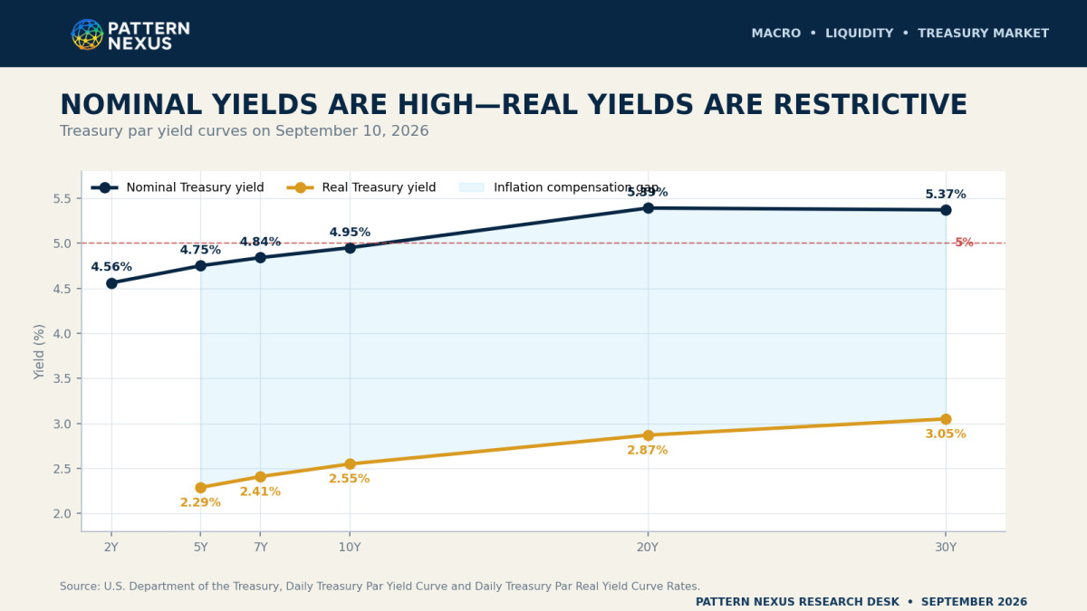
- The long end is already sitting directly beneath my stress thresholds. On September 10, the 10-year Treasury closed at 4.95%, the 20-year at 5.39%, and the 30-year at 5.37%. The corresponding real yields were 2.55%, 2.87%, and 3.05%.[1][2]
- The Fed expanded Treasury holdings, but almost all of the yearly increase came through bills. Treasury holdings were $4.552 trillion on September 9, up $351.4 billion from a year earlier, while bill holdings alone were up $352.9 billion. The Fed repaired reserve plumbing. It did not remove the duration the private market is being forced to carry.[4]
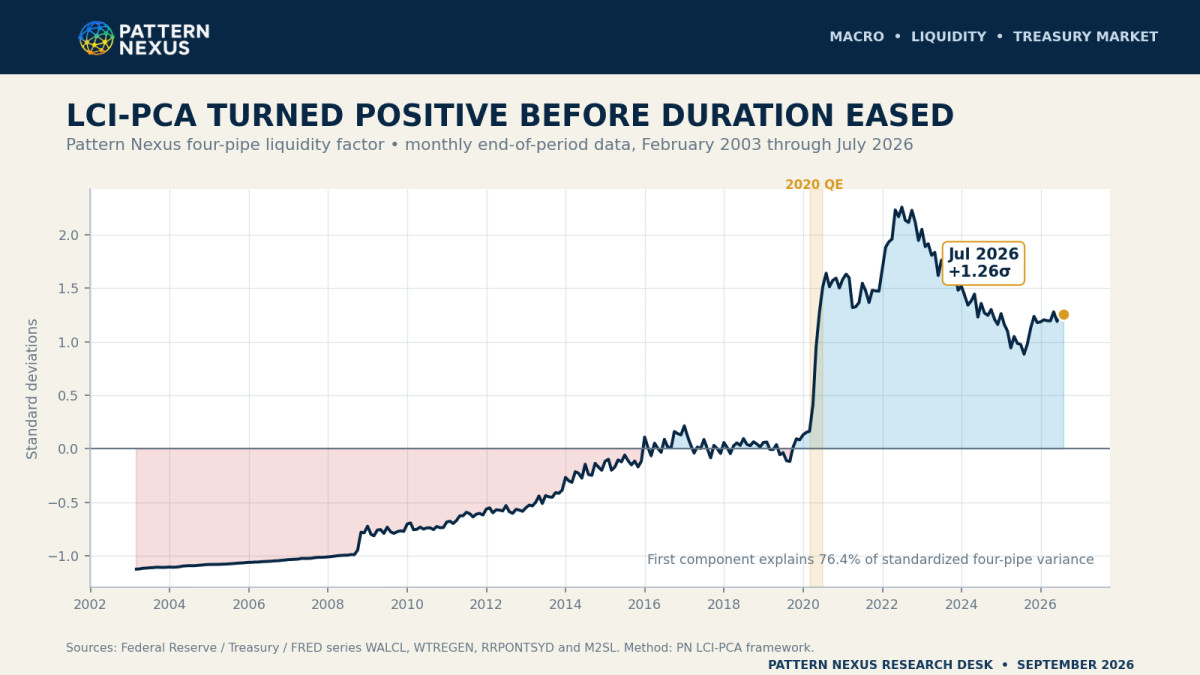
- The formal LCI-PCA liquidity factor remains positive at approximately +1.26 standard deviations through July 2026. Fed assets, the exhausted RRP reservoir, and M2 support the regime, while the TGA is the primary active drain. Positive liquidity and restrictive duration are coexisting because the liquidity is concentrated at the front end.[15][22]
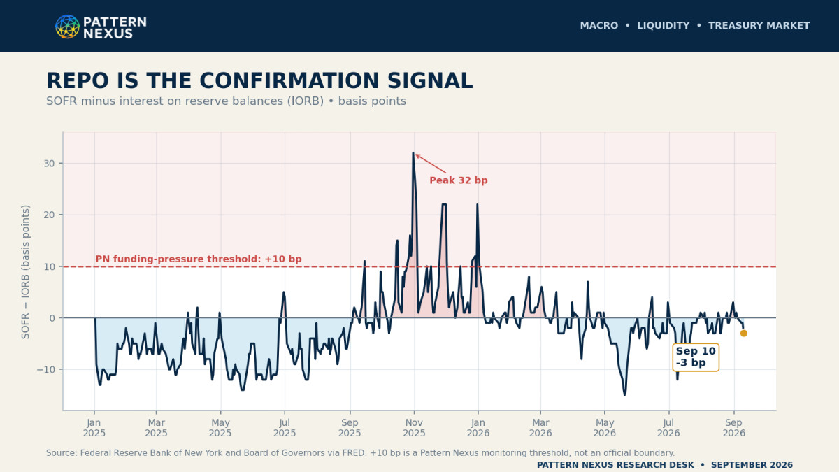
- Repo is not confirming a break yet. SOFR ended September 10 three basis points below IORB. That keeps the immediate probability of direct coupon QE below 50%, but the spread reached +32 basis points in late 2025, showing how quickly the funding layer can change around settlements and balance-sheet constraints.[22]
- The August CPI report makes the policy problem worse. Headline CPI rose 0.4% in one month and 3.4% over the year; energy rose 16.3% and gasoline 27.4%. Core inflation eased to 2.4% year over year, but rose 0.3% in August. This makes a conventional easing announcement harder even as it increases the pressure that may eventually force a market-functioning intervention.[3]
- Treasury has already begun the first line of defense. It doubled, at minimum, the size of long-end liquidity-support buybacks beginning September 9. That is not Fed QE, but it is direct evidence that the duration layer is now being managed rather than ignored.[8]
- The most important implementation window is late October through year-end, followed by the first half of 2027. Treasury expects the TGA could peak near $1.05 trillion in late October, October bill sizes are expected to rise, and the FOMC meets October 27–28 and December 8–9.[7][9]
- A yield breach alone is not enough. If the 10-year remains above 5.00% or the 30-year moves above 5.50% while auctions, repo, dealer balance sheets, or leveraged Treasury trades begin malfunctioning, my conditional probability of a larger intervention rises above 85%.
This report joins the full Pattern Nexus liquidity framework, the LCI-PCA liquidity composite, the QE 2026 forecast record, Treasury issuance and buybacks, Federal Reserve reserve-management purchases, real and nominal yield pressure, the newest CPI release, funding-market leverage, and the September 10 unstable-barbell scenario tree. It separates what has already happened from what has not, derives the intervention probabilities transparently, maps the likely program in stages, and identifies the dates and market conditions that can force each stage into existence.
The Fed fixed the plumbing. The long end is now testing whether the repair was enough.
I have spent most of the past year writing that 2026 would be the next balance-sheet expansion cycle. The original argument was never simply that the Fed would wake up one morning, announce another pandemic-sized QE program, and start buying everything. The argument was that the system would run out of room to continue shrinking. The reverse-repo cushion would disappear. Treasury issuance would keep growing. Reserve demand would collide with the floor system. The names would change, the tools would evolve, but the balance sheet would have to expand again.
That part happened.
QT ended. Reserve-management purchases began. The Fed’s Treasury holdings rose by more than $350 billion over the year. MBS principal was redirected into Treasury bills. The system got the reserves it needed, and the short-end plumbing remained orderly.
But the 10-year is now 4.95%. The 30-year is 5.37%. The real 30-year is above 3%. Mortgage rates are still crushing turnover. Treasury is doubling long-end buybacks. Inflation is still too high for the Fed to openly declare victory and ease. That combination creates the next phase of the problem.
Phase one was reserve support. Phase two is duration absorption.
The question is no longer whether the balance sheet expands from its QT low. It already did. The question is whether bills and reserve plumbing can remain separated from the long end while trillions of dollars in government debt, AI infrastructure, housing finance, private credit, and refinancing demand compete for the same duration capacity.
My answer is that the separation can survive for a while, but probably not indefinitely. The broader intervention architecture has about a 70% chance of expanding materially within six to twelve months. Direct Fed duration purchases have about a 40% to 45% chance in that window. If the long end crosses my red zone and market functioning begins to fracture, the probability rises rapidly from a forecast into a mechanical response.
The core call: QE 2026 is not starting from zero. It is moving from a confirmed reserve-management phase toward a probable duration-management phase. The policy may never be called QE, but the economic test is simple: does the public sector create reserves, shorten the duration private markets must absorb, or purchase that duration outright? If the answer becomes yes, the label is secondary.
Phase one is already here
The Fed is no longer shrinking Treasury holdings. It added bills to rebuild and maintain reserves. The forecast has moved from whether expansion begins to how far out the curve it must travel.
Liquidity quantity is not liquidity routing
The LCPI can rise while the long end remains tight. Bills, reserves, money funds, stablecoins, and short collateral can be liquid while mortgages, project finance, and Treasury duration remain expensive.
Inflation can force a two-direction policy
The Fed may have to remain restrictive at the policy-rate layer while becoming more supportive at the balance-sheet and market-functioning layers.
Treasury crossed the rhetorical line first
It is already calling the operations “long-end liquidity support” and doubling their size. That is not QE, but it confirms where the pressure has migrated.
01 · THE CONFIRMED PHASE
Phase one of QE 2026 is no longer a forecast
Before estimating the next intervention, I need to separate the part of the call that has already happened from the part that remains unresolved.
In The Calm Before the Liquidity Storm, I laid out a sequence: repo support, the end of QT, then a renewed liquidity-expansion phase operating through a more modern set of rails.[17] In QT Ends, Liquidity Returns, I argued that the system had reached the point where balance-sheet growth was becoming maintenance rather than optional stimulus.[13]
The Federal Reserve officially distinguishes reserve-management purchases from large-scale asset purchases. That distinction matters for policy communication, but it does not erase the balance-sheet mechanics. The New York Fed says reserve-management purchases are designed to maintain ample reserves and are not a change in the monetary-policy stance. It also explicitly contrasts them with crisis-era purchases of longer-term securities.[10]
That is almost exactly the distinction I have been making. Phase one is not long-duration QE. It is permanent balance-sheet maintenance inside an ample-reserves system.
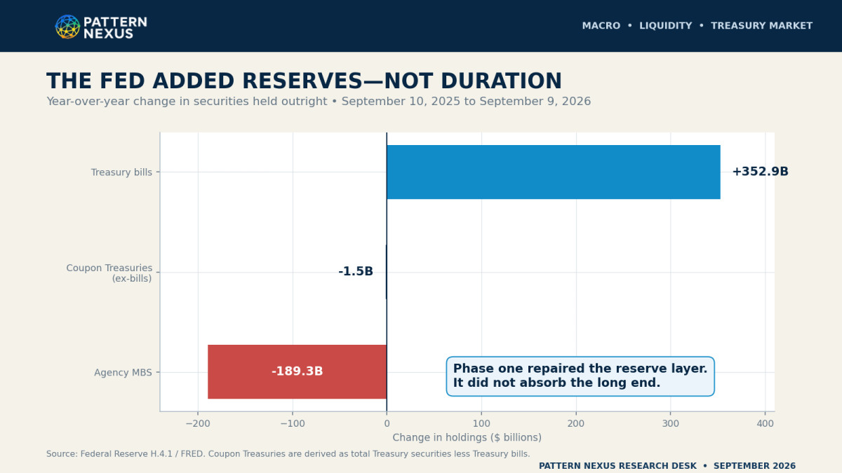
As of September 9, Federal Reserve Treasury holdings stood at $4.552 trillion, up $351.4 billion from the same week a year earlier. Bill holdings were $548.4 billion, up $352.9 billion. Nominal notes and bonds were up only $36.1 billion, while inflation-indexed holdings and inflation compensation declined. MBS holdings were down $189.3 billion.[4]
The composition is the entire story. The Fed expanded the Treasury side of its portfolio, but the increase was concentrated almost perfectly in bills. It created reserves and replaced MBS runoff with short Treasury collateral. It did not meaningfully bid for the 10-, 20-, or 30-year duration currently bearing the pressure.
Balance-sheet size and balance-sheet duration are not the same policy
This is where most of the public QE argument gets flattened. A dollar of bill purchases and a dollar of 30-year bond purchases both add a dollar of assets to the Fed’s balance sheet, but they do not remove the same risk from the market. A bill has almost no price sensitivity to a change in long rates. A 20- or 30-year coupon carries years of duration, convexity, financing exposure, and mark-to-market volatility. The accounting amount can be identical while the market effect is completely different.
That is why I separate reserve creation from duration absorption. Reserve-management purchases change the quantity and distribution of reserves. Coupon purchases change who carries interest-rate risk. Operation Twist changes the maturity composition even if the headline balance-sheet total barely moves. Full QE does both: it creates reserves and removes duration.
The latest portfolio data make that separation visible. From September 2025 to September 2026, the Fed’s bill book grew by roughly $352.9 billion. Coupon Treasuries excluding bills changed by only about negative $1.5 billion on net, while agency MBS fell by roughly $189.3 billion. In other words, the balance sheet expanded, but its new support was concentrated at the front end. The long end was still left to clear through Treasury auctions, dealers, foreign buyers, pensions, insurers, banks, hedge funds, households, and leveraged relative-value trades.
This is why calling every balance-sheet increase “the same QE” is analytically useless. The right question is not only how large the Fed becomes. It is what maturity risk disappears from private hands because the Fed became larger.
The New York Fed’s monthly schedule makes the sequence even clearer. Reserve-management purchases ran near $40 billion per month early in 2026, slowed to $25 billion, then $10 billion, and fell to zero for the August 14 through September 14 period. Reinvestment purchases continued at approximately $17 billion.[5]
This is not evidence that the liquidity cycle disappeared. It is evidence that the first reserve rebuild was sufficient to calm the short end for now. Weekly average reserves rose to $2.991 trillion in the latest H.4.1 release, while the TGA fell by $84.6 billion to $883.3 billion. The Wednesday point observations were $3.037 trillion in reserves and $843.7 billion in the TGA.[4]
That reserve bounce did not come from a new wave of Fed purchases. It came mainly from money leaving the Treasury’s account and returning to the banking system. The balance sheet’s liability mix changed. That is why the system can look comfortable today and still tighten sharply when Treasury refills the TGA.
Phase one answered the reserve-floor question. It did not answer the duration-capacity question.
02 · THE LIQUIDITY COMPOSITE
What the LCPI is saying—and what the long end adds to it
The Pattern Nexus liquidity composite was built because looking at the Fed balance sheet alone is not enough. The published LCI-PCA framework combines the Fed’s balance sheet, the TGA, the reverse-repo facility, and M2 after aligning and standardizing the series, with TGA and RRP inverted because increases in those reservoirs generally absorb liquidity from the private system.[14][15]
The formal construction matters
The index is not built by placing four raw lines on one chart and deciding which one looks most important. Each series arrives at a different frequency and in a different unit. WALCL and the TGA are weekly. ON RRP is daily. M2 is monthly. One is measured in trillions, another can move by tens of billions in a week, and two of the four pipes operate in the opposite direction from their raw level.
The published method solves that problem in four steps. First, each series is converted to month-end using the last available observation. Second, slower series are carried forward so all four pipes share the same date. Third, WALCL and M2 retain their normal sign while the TGA and RRP are inverted. Fourth, every aligned series is standardized into a z-score before the first principal component is extracted.[15][16]
The four aligned inputs: WALCL, −TGA, −ON RRP, and M2.
The equal-weight cross-check: LCI-EW = (ZWALCL + Z−TGA + Z−RRP + ZM2) ÷ 4.
The statistical core: LCI-PCA is the first principal component of those four standardized, direction-aligned series, with the sign anchored so a higher factor means a more liquidity-positive regime.
For this report, I use LCI-PCA for the reproducible statistical core and LCPI for the live Pattern Nexus pressure reading built around it. The LCI-PCA tells us whether the base liquidity machine is expanding, flattening, draining, or bottoming. The wider LCPI interpretation adds the transmission layer: reserves, repo, collateral velocity, real yields, Treasury duration, auction capacity, and where the liquidity is actually landing.
That distinction matters because the index is a regime tool, not a daily trading signal. I do not splice a partial September M2 estimate into a monthly PCA series just to make it look current. The formal common-data reading ends in July 2026, the latest month available across all four inputs. The September reserve, TGA, RRP, and rate data are then read as the live plumbing overlay.
I have also expanded the conceptual framework to account for stablecoins, Treasury-backed digital liquidity, money-market funds, repo capacity, and collateral looping. Those channels can create a much larger usable liquidity surface than the narrow reserve number alone suggests. One bucket can feed many hoses. The same short Treasury can support a money fund, a repo transaction, a stablecoin reserve, a derivative margin process, and a collateral chain.
That is why the LCPI regime signal can turn positive before every part of the economy feels easier. Liquidity is not evenly sprayed across the system. It enters through specific pipes, touches specific collateral, and is captured first by the balance sheets closest to those pipes.
Right now, the reserve and short-collateral layers are relatively liquid. Bills have buyers. Money markets are functioning. The Fed has an explicit mechanism to replenish reserves. Stablecoin and tokenized-Treasury rails create additional structural bill demand. But the system is not equally liquid at ten, twenty, or thirty years.
This is the distinction I formalized in the September 10 report, Two Economies, One Balance Sheet: the economy is liquid at the reserve layer, tight at the duration layer, profitable at the capital layer, and fragile at the household cashflow layer.[12]
The LCPI tells me the system has entered a renewed liquidity regime. The long-rate overlay tells me whether that liquidity is reaching the duration-sensitive economy.
The latest four-pipe reading is supportive, but not uniform
The July 2026 z-scores show the internal split clearly. Fed total assets were about +1.06 standard deviations relative to the 2003–2026 sample. Inverted ON RRP was approximately +0.46 because the old multi-trillion-dollar RRP reservoir has largely emptied back into the market. M2 was roughly +1.85. Inverted TGA, however, was about −1.64, making Treasury’s cash account the major active drain.
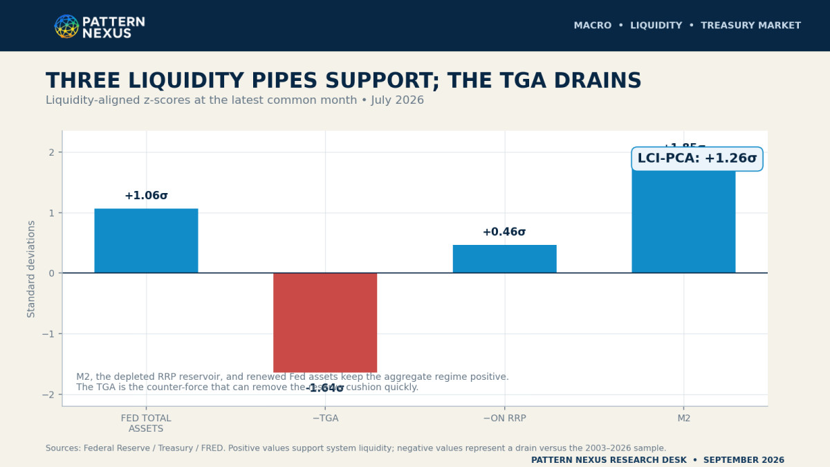
This is the setup beneath the QE probability. The system does not begin from a pure liquidity drought. It begins from a positive but badly routed regime. M2 and the Fed’s balance sheet support the broad collateral machine. The disappearance of the RRP reservoir released a large stock of cash into bills and repo. The TGA can still pull reserves out quickly. None of those conditions guarantees that a 30-year bond clears at a price compatible with housing, fiscal arithmetic, regional-bank balance sheets, or long-lived infrastructure.
That is also why a rising LCPI does not automatically mean the Fed can ignore the long end. The composite measures the state of the liquidity machine. It does not promise that every maturity, institution, or household receives the same transmission. Liquidity can be abundant in one layer and scarce in another. The current system is proving that in real time.
| System layer | Current condition | What it means |
|---|---|---|
| Bank reserves | Ample, but flow-sensitive | The latest level is comfortable, but a TGA rebuild can drain it quickly. |
| Bills and short collateral | Supported | Fed purchases, money funds, bank liquidity demand, and digital-dollar reserves create buyers. |
| Coupon Treasuries | Under pressure | Private markets still absorb most of the real-rate and term-premium risk. |
| Housing and mortgages | Restrictive | Long rates are suppressing turnover and refinancing even without a banking crisis. |
| AI and large-cap capital | Still funded | Profits, equity valuations, private credit, banks, and infrastructure finance support the buildout. |
| Household cashflow | Fragile | Inflation and financing costs absorb income before reserve liquidity reaches households. |
The LCPI is not failing because the 10-year is high. It is showing the regime correctly. The missing variable is routing. The present system is producing liquidity that prefers bills, collateral, digital rails, and high-quality capital while leaving the private market to price duration.
03 · THE ACTIVATION ZONE
The long end is no longer approaching the line—it is sitting on it
On September 10, the Treasury curve closed with the 2-year at 4.56%, the 5-year at 4.75%, the 7-year at 4.84%, the 10-year at 4.95%, the 20-year at 5.39%, and the 30-year at 5.37%.[1]
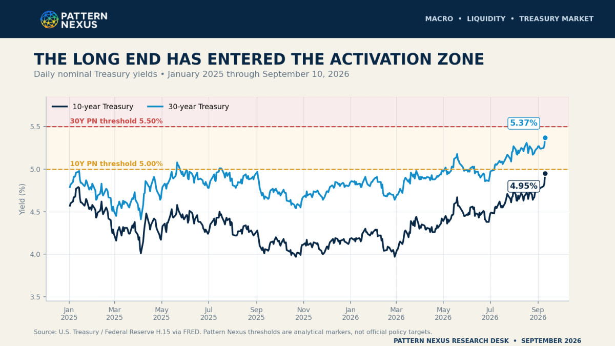
The 10-year is five basis points below the 5.00% threshold in my stress dashboard. The 30-year is thirteen basis points below 5.50%. Those are not magical numbers. Nothing mechanically breaks because a screen changes from 4.99 to 5.00. They are boundary markers for a region in which the cost of carrying duration begins transmitting faster into housing, project finance, Treasury interest expense, bank securities portfolios, leveraged Treasury trades, and the political system.
The real curve is even more important. On the same date, the real 5-year was 2.29%, real 7-year 2.41%, real 10-year 2.55%, real 20-year 2.87%, and real 30-year 3.05%.[2] This is not simply a story about inflation expectations blowing out. Real required returns are doing the tightening.
Why the 10-year matters before anything visibly breaks
The 10-year is the center of the private financing system. It is not a direct setting on a mortgage application, a commercial-real-estate loan, or a project-finance term sheet, but it is embedded in the benchmark curve used to price all of them. When it moves from the low fours toward 5%, lenders do not merely add the same fifty or seventy-five basis points to every borrower. Credit spreads can widen with it, hedging costs change, bank risk limits tighten, and the monthly payment jumps faster than the Treasury screen alone suggests.
That is why 5% is a transmission threshold rather than a mystical number. It is where a high nominal benchmark, a high real benchmark, and an already expensive credit spread begin stacking on top of each other. The economy can survive that price for a day or a month. The question is whether it can refinance into it repeatedly while Treasury issuance keeps adding supply.
Why the 30-year tells me whether duration capacity is failing
The 30-year contains the largest concentration of term-premium, inflation, fiscal, and convexity risk on the nominal curve. A buyer is not lending to the government for one business cycle. The buyer is accepting decades of uncertainty over inflation, deficits, taxation, issuance, productivity, war, energy, currency value, and the future reaction function of the Federal Reserve.
At 5.37%, with a real yield of 3.05%, the 30-year is telling us that investors are demanding a large inflation-adjusted return to warehouse that uncertainty. If the nominal yield moves through 5.50% while the real yield remains above roughly 3.10%, the problem is no longer only that “rates are high.” The market is saying the marginal balance sheet requires a materially lower price before it accepts another unit of duration.
The private sector is carrying four duration forces at once
- Net Treasury coupon supply: persistent deficits require continuing issuance across notes and bonds.
- Mortgage convexity: when rates rise, expected mortgage duration extends because fewer borrowers refinance. Investors who thought they owned a shorter asset suddenly own a longer one and may hedge by selling Treasuries or paying fixed rates.
- Dealer inventory and auction settlement: dealers must finance securities they cannot immediately distribute, using balance sheet that becomes more expensive as volatility rises.
- Leveraged relative-value demand: hedge funds can absorb Treasuries through repo-funded basis and swap-spread trades, but that demand reverses quickly if financing or margin changes.
Those forces can all be manageable separately. The danger is synchronization. Larger coupon auctions raise dealer inventory. Higher yields extend mortgage duration. Higher volatility increases hedge requirements. Repo lenders demand more margin. The leveraged buyer that helped clear yesterday’s auction can become tomorrow’s forced seller.
That is the exact problem I have described in the fiscal-dominance and gravity-zone work. When deficits remain large, interest expense compounds, the private sector must absorb continuing coupon supply, and real capital demand stays firm, the long end can resist the policy rate. The Fed can stop QT, add bills, or even cut the overnight rate and still fail to deliver meaningful relief to mortgages or long-duration borrowers.[19][20]
I need to be direct about the earlier rate call. My expectation that the 10-year would eventually fall below 3% did not happen on the timing or level I expected. The long end stayed much higher. Treasury supply, fiscal pressure, real yields, war and energy risk, and AI-linked capital demand overpowered the disinflationary forces I expected to dominate sooner. I have already documented that miss in the public call audit.[21]
But that miss does not weaken the liquidity-intervention thesis. It changes its mechanism. If the 10-year will not fall naturally, and if the government, housing market, AI buildout, banking system, and refinancing structure cannot comfortably live with it near 5%, the probability shifts from conventional rate relief toward balance-sheet and duration management.
The long-end miss is not something to erase. It is the reason phase two has become more probable.
04 · THE INFLATION TRAP
The CPI report delays obvious QE while increasing the need for disguised support
The August CPI report arrived at exactly the wrong moment for a central bank facing long-end stress. Headline CPI rose 0.4% in August, accelerating from 0.1% in July, and remained 3.4% above its year-earlier level. Energy rose 2.1% during the month and 16.3% over the year. Gasoline rose 3.9% in August and 27.4% over twelve months. Core CPI increased 0.3% for the month and 2.4% over the year.[3]
The report contains both an inflationary and a disinflationary signal. Core inflation is lower than headline and eased slightly on a twelve-month basis. Shelter inflation is slowing compared with the prior cycle. But the monthly headline acceleration, energy shock, and renewed shelter increase are enough to keep the Fed constrained.
The July FOMC minutes already showed that constraint. Three voters preferred a 25-basis-point rate increase. Many participants believed additional tightening could become necessary if inflation failed to decline. The same minutes said hedge-fund leverage remained near all-time highs, repo and prime-brokerage borrowing had risen to record levels, and Treasury-market volatility could threaten financial stability.[6]
This creates what looks like a contradiction only if monetary policy is treated as one lever.
The Fed can hold or raise the policy rate to maintain an anti-inflation stance while expanding reserves to protect money-market control. It can support Treasury-market functioning without describing the action as economic stimulus. It can alter the maturity composition of its holdings while arguing that the federal-funds rate remains the primary signal of monetary-policy stance.
In other words, the Fed can tighten the price of short money while loosening the quantity and routing of balance-sheet support.
| Policy layer | Possible action | Official message | Economic effect |
|---|---|---|---|
| Policy rate | Hold or raise | Inflation remains elevated | Maintains restrictive short-rate signal |
| Reserve layer | Resume RMPs | Maintain ample reserves | Adds reserves and protects rate control |
| Funding layer | Expand repo operations | Support market functioning | Prevents forced deleveraging |
| Portfolio layer | Change maturity composition | Improve implementation or resilience | Moves public support farther out the curve |
| Duration layer | Buy coupon Treasuries | Temporary market-functioning operation | Removes duration from private balance sheets |
The new CPI report therefore has two opposite timing effects. It reduces the chance that the Fed announces conventional QE at the September meeting. At the same time, it increases the chance that long yields remain high, rate cuts remain unavailable, and the Fed is eventually forced to use balance-sheet tools that it can separate rhetorically from the policy stance.
Inflation delays the label. It increases the medium-term pressure behind the mechanism.
05 · PROBABILITY METHOD
How I moved from a framework to a probability
These numbers are not presented as a machine-generated certainty or an official forecast. They are conditional probabilities built from the four-branch scenario tree in the September 10 report, updated for the September 10 Treasury close, the latest H.4.1 balance sheet, Treasury’s long-end buyback expansion, and the August CPI release.
The earlier scenario tree assigned 38% to controlled compression, 30% to a stagflationary squeeze, 20% to a duration or credit break, and 12% to a broad AI-led reflation. The new CPI report and the move in real yields shift the tree modestly. I now assign:
| Six-to-twelve-month branch | Updated weight | Core condition |
|---|---|---|
| Controlled compression | 34% | Inflation and long real yields ease without a credit accident. |
| Stagflationary squeeze | 34% | Inflation blocks meaningful cuts while long rates and household pressure remain high. |
| Duration or credit break | 22% | Yields, auctions, funding, leverage, or credit produce a recognizable market-functioning event. |
| Broad AI-led reflation | 10% | Growth and productivity broaden enough to absorb high real rates without immediate intervention. |
I then estimate the conditional probability of each policy response inside each branch.
| Branch | Larger QE-like architecture | Fed coupon-duration purchases | Full emergency QE |
|---|---|---|---|
| Controlled compression | 50% | 15% | 5% |
| Stagflationary squeeze | 85% | 50% | 15% |
| Duration or credit break | 100% | 95% | 75% |
| Broad AI-led reflation | 20% | 5% | 2% |
Weighting those conditional outcomes by the scenario probabilities produces approximately 70% for a broader QE-like architecture, 43.5% for direct Fed coupon-duration support, and roughly 23% to 25% for full emergency QE over the next six to twelve months.
The weighted math behind the headline number
The 70% is not a confidence score I attached to a narrative. It is the sum of four conditional paths. Controlled compression contributes 17.0 percentage points: a 34% branch weight multiplied by a 50% probability of some larger QE-like support inside that branch. The stagflationary squeeze contributes 28.9 points. A duration or credit break contributes 22.0 points. Broad AI-led reflation contributes 2.0 points. Together they produce 69.9%, which I round to 70%.
The same calculation produces 43.5% for meaningful Fed coupon-duration purchases: 5.1 points from controlled compression, 17.0 from the stagflationary squeeze, 20.9 from a duration or credit break, and 0.5 from broad reflation. Full emergency QE comes out near 23.5%, with most of that tail risk concentrated in the duration-break branch.
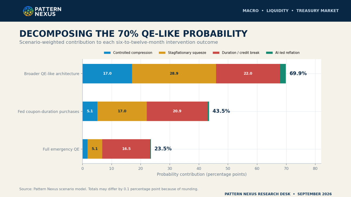
This structure prevents two common errors. The first is treating all forms of intervention as one binary event. Treasury buybacks, reserve-management purchases, term repo, Operation Twist, coupon purchases, and full QE are different steps with different political costs and different effects on duration. The second is treating the scenarios as if they were completely isolated. The economy can begin in stagflation, move into weak auctions, trigger a basis-trade unwind, and end in emergency QE. The branches describe the path into the response; they do not prevent one path from becoming another.
The scenario model is also why the high inflation print does not automatically lower the QE probability. It lowers the probability of an easy, discretionary, openly dovish program. At the same time, it raises the probability of a two-track regime in which the Fed keeps the policy rate restrictive but is forced to support market functioning through the balance sheet. Inflation changes the label and timing before it changes the mechanical need.
This also explains why the probability of “something larger” is much higher than the probability of a 2020-style QE announcement. Treasury buybacks, bill-heavy issuance, reserve-management purchases, reinvestment changes, term repo, regulatory adjustments, and an Operation Twist structure can all be expanded before the Fed announces an open-ended asset-purchase program.
06 · THE PROBABILITY MAP
The probability rises sharply with time because the balance-sheet need is structural
The probability is not static. It compounds as Treasury debt rolls over, currency and other Federal Reserve liabilities grow, the TGA moves, MBS runoff changes the portfolio, long-duration financing resets, and private balance sheets absorb additional coupon supply.
| Cumulative probability | By December 2026 | By mid-2027 | By end-2027 |
|---|---|---|---|
| Material expansion of the QE-like architecture | 45% | 70% | 82% |
| Fed purchases move materially beyond bills and short notes | 30%–35% | 50%–55% | 65%–70% |
| Full emergency QE program | 15%–20% | 30% | 40%–45% |
| Explicit hard yield-curve control | Below 5% | About 10% | 15%–20% |
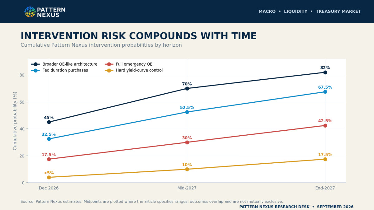
These outcomes overlap. A program can begin as reserve management, move into portfolio composition, add term repo, and later become full QE. The table is cumulative, not a set of mutually exclusive bets.
Why the curve steepens with time
Every month without a clean decline in real long yields moves more debt and more private financing toward a higher reset rate. Treasury securities mature and must be refinanced. Corporate debt rolls. Commercial mortgages reach extension decisions. Utilities and data-center projects move from planning into funded construction. Banks continue carrying securities purchased in an older rate regime. MBS runoff keeps reducing one of the Fed’s largest duration positions unless the reinvestment policy changes.
The probability therefore rises even if no single crisis date arrives. A stable 5% 10-year is not neutral simply because it becomes familiar. Time converts the market price into cash expense. Cash expense becomes budget pressure, debt-service pressure, reduced lending, weaker coverage ratios, and eventually political pressure. That slow transmission is why the six-month and eighteen-month probabilities are materially different.
Hard yield-curve control remains the least likely branch because it commits the Fed to defend a visible number. A softer state-contingent program can achieve much of the same result without declaring a permanent ceiling. That is why the probability of functional duration control rises far faster than the probability of an explicit cap.
The headline probability I would publish today is therefore straightforward:
There is a 70% probability that the QE-like architecture is materially expanded within six to twelve months, and a 40% to 45% probability that the Fed itself is forced into meaningful duration purchases during that window.
The probability of an explicit program called “quantitative easing” is much lower. The probability of the economic substance appearing under several separate names is much higher.
07 · TREASURY MOVES FIRST
The first duration intervention is already operating outside the Fed
In November 2025, I wrote The Treasury Just Drew Its Line in the Sand—And It’s at the 10-Year.[18] The point was not that Treasury could permanently peg the 10-year by itself. The point was that debt management was becoming an active part of the monetary operating system.
That shift is now visible in official language. On August 19, Treasury announced that it would increase by at least double the size of its “long-end liquidity support buybacks” beginning September 9. Operations in the 10-to-20-year and 20-to-30-year sectors moved from a $2 billion maximum to at least $4 billion per operation.[8]
Treasury’s August refunding statement also authorized up to $38 billion of liquidity-support buybacks across maturity buckets during the quarter, plus up to $25 billion of short-maturity cash-management buybacks. It maintained coupon auction sizes for the next several quarters while stating that October bill sizes were expected to rise.[7]
Buybacks help in three ways. They remove less-liquid off-the-run securities, improve price discovery, and allow Treasury to manage the maturity and liquidity profile of outstanding debt. If they are financed with bills, they also shorten the effective duration the private sector must hold.
But Treasury cannot create reserves. It can swap one security for another, change issuance composition, and redistribute duration. Only the Fed can expand the monetary base and remove duration from private balance sheets at scale.
That means Treasury is the first line of defense, not the final line. If doubled buybacks and bill-heavy financing stabilize the long end, the Fed may never need to announce a large coupon program. If those measures fail, they become the bridge to Fed involvement.
Watch the language: Treasury is no longer merely conducting generic buybacks. It is explicitly increasing “long-end liquidity support.” That is the government identifying the problem before the Fed identifies it as a monetary-policy problem.
08 · PROGRAM DESIGN
What the next intervention will probably look like
The most likely program is not one announcement. It is a ladder. Each rung is politically and institutionally easier than the one above it. Authorities climb only as high as the market forces them.
Stage 0: the existing reserve-management system
This is already active. The Fed rolls over Treasury principal, reinvests agency principal into Treasury bills, and can purchase bills—or securities with remaining maturities of three years or less—when needed to maintain ample reserves. The current directive already authorizes this short-duration expansion.[5][6]
The first visible confirmation of renewed pressure would be a return of monthly RMPs after the current zero-purchase period. My expected initial pace would be approximately $20 billion to $40 billion per month, scaled around TGA movements, currency growth, reserve demand, and money-market conditions. That is my estimate, not an announced amount.
Stage 1: Treasury expands the duration shield
Treasury can raise the size or frequency of 10-to-30-year buybacks, shift more net financing toward bills, reduce the relative long-coupon share of future borrowing, and use cash-management operations to smooth settlement pressure. This stage is already beginning.
A realistic next move would be repeated $6 billion to $10 billion long-end liquidity operations, or more frequent operations at the present $4 billion-or-greater size. Treasury could frame every step as market-liquidity management rather than yield suppression.
Stage 2: term funding and dealer-capacity support
If repo or leveraged Treasury positions become the transmission channel, the Fed can expand standing repo access, add temporary 7-, 14-, 28-, or 42-day operations, broaden counterparties, and coordinate regulatory changes that free dealer balance-sheet space. The goal would be to stop forced selling before it becomes a full duration event.
This is especially relevant because the July minutes described hedge-fund leverage near record highs and repo and prime-brokerage borrowing at record levels. High leverage can remain invisible while volatility is low. The problem appears when margin, financing, or market depth changes at the same time.[6]
Stage 3: an Operation Twist or portfolio-composition program
This is the most probable bridge between reserve management and full QE. The Fed could allow bills or short holdings to mature while reinvesting into 5-to-10-year and longer coupon securities. It could redirect MBS principal farther out the Treasury curve. It could keep the headline size of the balance sheet relatively stable at first while materially increasing the duration removed from the market.
The July FOMC minutes matter here. Most participants discussed balance-sheet policy, referenced a task force, and explicitly identified “the appropriate maturity composition” of Treasury holdings as an issue for future meetings.[6]
That is not an announcement. It is preparatory architecture. Central banks do not usually begin discussing maturity composition in detail because nothing may ever require it.
Stage 4: market-functioning purchases of coupon Treasuries
If long-end liquidity deteriorates, the Fed can authorize purchases across the 5-to-30-year curve. The first program would probably be targeted, temporary, and capped. My base design estimate is a $300 billion to $500 billion initial envelope, implemented at roughly $50 billion to $100 billion per month and weighted toward the 7-to-10-year and 20-to-30-year sectors.
The exact size matters less than the reaction function. If purchases are tied to auction performance, market depth, volatility, or funding spreads, the program becomes a soft backstop without an explicit yield target.
Stage 5: full QE
If duration stress spills into credit, banking, housing, or the leveraged Treasury complex, the temporary envelope can become open-ended. The Fed would reinvest maturities, purchase coupons across the curve, potentially add MBS if mortgage transmission becomes central, and activate swap or funding lines if dollar stress becomes global.
This is the lowest-probability high-impact branch over the immediate horizon, but it is the branch in which the response becomes largest fastest.
Stage 6: soft yield-curve control before hard yield-curve control
I do not expect the Fed to announce a permanent 10-year yield cap unless the system is already in a severe break. Hard yield-curve control makes fiscal dominance too visible and forces the central bank to defend a number against potentially unlimited selling.
A soft corridor is more likely. The Fed can refuse to name a target while purchasing more aggressively whenever yields, volatility, or market depth move beyond an internal pain range. Functionally, that is yield suppression. Institutionally, it is market-functioning support.
| Stage | Likely public label | Core mechanism | Balance-sheet effect |
|---|---|---|---|
| 0 | Reserve-management purchases | Bills and securities under three years | Expands reserves |
| 1 | Liquidity-support buybacks | Treasury removes off-the-run coupons | Changes public-debt composition |
| 2 | Temporary funding operations | Term repo and dealer support | Prevents forced deleveraging |
| 3 | Portfolio-composition adjustment | Twist from short holdings into coupons | Adds duration absorption without immediate net expansion |
| 4 | Treasury-market-functioning purchases | Targeted 5-to-30-year purchases | Expands balance sheet and removes duration |
| 5 | Financial-stability asset purchases | Open-ended Treasury and possibly MBS buying | Full QE mechanics |
| 6 | Market-resilience backstop | State-contingent purchases near an internal pain range | Soft yield-curve control |
The initial size will be chosen by the malfunction, not by one headline number
The face value of purchases is not the full policy signal. Forty billion dollars of bills and forty billion dollars of 30-year bonds are equal on an accounting statement, but the second operation removes vastly more duration and market risk. A serious program would therefore be calibrated by maturity, duration-equivalent exposure, auction needs, market depth, and the speed at which dealers can redistribute inventory—not only by the monthly dollar amount.
| Problem being repaired | Pattern Nexus base design estimate | Likely maturity focus | What confirms escalation |
|---|---|---|---|
| Reserve maintenance | $20B–$40B per month when needed | Bills to three years | Reserves fall with TGA growth or currency demand |
| Treasury liquidity shield | $6B–$10B per long-end buyback operation, or greater frequency | 10–20 and 20–30 years | Off-the-run liquidity and dealer inventories deteriorate |
| Portfolio composition / Twist | $250B–$400B maturity shift over six to nine months | Sell or run off bills; buy 5–30-year coupons | Long rates stay high while reserve conditions remain adequate |
| Targeted market-functioning purchases | $300B–$500B initial envelope; $50B–$100B per month | 7–10 and 20–30-year sectors | Repeated auction, depth, volatility, or funding failures |
| Full emergency QE | Open-ended; likely begins above $100B per month across assets | Broad coupon curve and potentially MBS | Treasury dysfunction transmits into banking, housing, or credit |
Those are analytical design ranges, not leaked plans or official forecasts. Their purpose is to show the scale transition. The Fed can solve a reserve-maintenance problem with tens of billions in bills. It may need hundreds of billions in maturity transformation to change the marginal price of duration. If a leveraged unwind is already moving hundreds of billions of exposure through a thin market, a tiny symbolic purchase program can fail before the first month is complete.
Where the Fed would probably concentrate purchases
The 7-to-10-year sector is the most likely first target because it contains the benchmark point connecting Treasury financing, mortgage pricing, corporate borrowing, and global portfolio hedging. The 20-to-30-year sector is the pressure valve because that is where fiscal, inflation, and convexity risk become hardest to warehouse. Buying both allows the Fed to address transmission and market function without announcing a permanent cap at one maturity.
MBS would probably remain secondary at the beginning. The Fed has spent years allowing the mortgage book to run down, and a return to MBS purchases would look like an explicit attempt to subsidize housing. But if Treasury purchases lower benchmark yields while mortgage spreads remain abnormally wide, or if convexity hedging becomes part of the Treasury selloff, MBS can reenter the program. The institutional justification would be transmission through housing finance rather than a housing rescue.
Operation Twist is the cleanest political bridge
A Twist structure lets the Fed say it is not increasing the total balance sheet even while it removes more duration from the market. Bills and short notes can mature or be sold while the Desk purchases longer coupons. Reserve creation can be neutralized at first, but private-sector duration still falls. That makes it the most politically attractive bridge when inflation remains above target and the long end is the specific malfunction.
The limitation is scale. The Fed does not hold an unlimited stock of bills that can be exchanged for long bonds, and selling the same short collateral demanded by banks, money funds, stablecoins, and repo participants can tighten the front end. If the market demands more duration absorption than the short book can finance, Twist turns into net expansion. That is the exact point where a program designed to avoid the appearance of QE becomes QE mechanically.
09 · TIMING
The calendar creates three increasingly dangerous windows
Window 1: September 15–16
The September FOMC meeting arrives four days after the August CPI release and less than a week after the Treasury curve moved to the edge of the red zone. I place only a 10% to 15% probability on an actual duration-purchase announcement at this meeting without a sudden market event.
The probability of preparatory language is much higher. The Committee can discuss the balance-sheet task force, maturity composition, Treasury-market resilience, reserve conditions, or the relationship between balance-sheet policy and financial conditions. It can also keep the policy rate restrictive while preserving flexibility over the Desk’s purchase authority.
Window 2: late October through early November
This is the first major implementation window. Treasury expects its cash balance to be about $950 billion at the end of September and potentially peak at $1.05 trillion, plus or minus $50 billion, in late October. October bill sizes are expected to rise. The FOMC meets October 27–28, and Treasury’s next quarterly refunding announcement arrives November 4.[7][9]
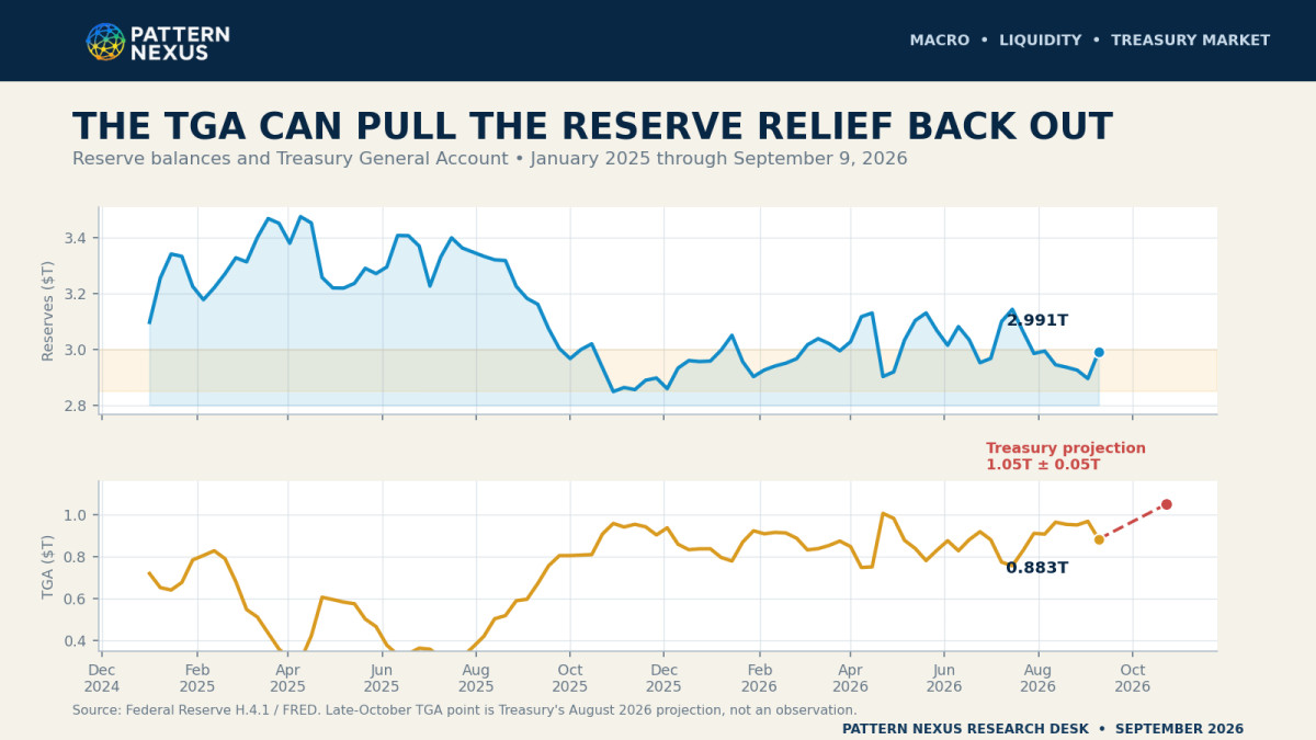
A rising TGA absorbs reserves. New bill issuance competes for cash. Coupon settlements use dealer balance sheet. If the 10-year and 30-year remain near or above the red zone during that sequence, the same week can produce reserve pressure, duration pressure, and political pressure.
The settlement sequence is what makes the window dangerous
The TGA is not an abstract accounting line. When Treasury issues debt and the proceeds accumulate in its Federal Reserve account, cash leaves private bank deposits and reserve balances move to the TGA. When Treasury spends, the direction reverses. That is why the latest weekly reserve bounce arrived beside an $84.6 billion decline in the TGA. The private system received cash because Treasury’s account released it.
Late October can run the mechanism in reverse. Treasury can increase bills, settle coupon auctions, and rebuild cash while the long end is already near the stress line. Money funds may absorb the bills easily, but that does not mean dealers and real-money buyers have unlimited capacity for the coupons. The short end can clear while the long end weakens. That is the same split the LCPI and duration overlay are already showing.
The sequence I am watching is therefore specific: TGA rises, reserves fall, SOFR begins trading persistently above IORB, auction tails become more frequent, dealers retain more supply, the 10-year holds above 5%, and the 30-year presses through 5.5%. None of those observations alone forces QE. Their overlap turns a restrictive rate environment into a market-functioning problem.
Window 3: December through the first half of 2027
Year-end compresses dealer balance sheets and makes funding conditions less forgiving. The December 8–9 FOMC meeting is the final scheduled policy window of 2026 and includes updated economic projections.[9]
If the system reaches year-end with long rates still near 5% and 5.5%, inflation still limiting rate cuts, and reserves moving lower again, the probability of a larger technical program rises sharply. If year-end passes without dysfunction, the first half of 2027 becomes the most likely period for the intervention to move from preventive to unavoidable.
December also matters because year-end balance-sheet reporting changes behavior. Dealers, banks, hedge funds, and foreign institutions reduce or reprice balance-sheet usage around reporting dates. A market that functions with plenty of intermediation in October can become far less elastic in the final weeks of the year. If a large Treasury settlement, a volatility shock, or a collateral demand spike lands inside that window, authorities have less time to pretend the problem is temporary.
The first half of 2027 is the stronger structural window because it allows the Fed and Treasury to exhaust the easier tools first. Treasury can expand buybacks. The Fed can restart reserve-management purchases. Term repo can be offered. Dealer-capacity rules can be adjusted. Reinvestment can be redirected. If long rates still refuse to compress after those steps, the argument for coupon purchases becomes much easier to make: the authorities tried technical plumbing first, and the market proved the binding constraint was duration.
| Window | Most likely action | What would accelerate it |
|---|---|---|
| September 2026 | Preparation, language, renewed RMP flexibility | Sudden auction, repo, or credit dysfunction |
| Late October–November | Larger RMPs, Treasury buybacks, funding support | TGA near $1 trillion plus long yields above thresholds |
| December 2026 | Term operations or portfolio-composition change | Year-end dealer and repo stress |
| First half 2027 | Targeted duration purchases | Persistent real yields, weak auctions, or credit transmission |
| Second half 2027 | Broader QE architecture | Failure of earlier stages to compress long rates |
10 · ACTIVATION DASHBOARD
The Fed does not intervene because a yield looks ugly. It intervenes when the yield begins breaking the machine.
The threshold has to be read as a system, not a single line on a chart. A 10-year at 5.05% with strong auctions, stable repo, deep markets, and healthy credit is restrictive, but not necessarily an emergency. A 10-year at 4.90% with collapsing depth, repeated auction tails, record leveraged positioning, and a widening funding basis can be much more dangerous.
Repo tells me whether duration stress has become funding stress
The cleanest daily confirmation is not simply the level of SOFR. It is how secured overnight funding trades relative to the Fed’s administered rates and whether the pressure persists beyond one settlement date. SOFR above the interest rate on reserve balances means private borrowers are paying more for Treasury-backed overnight cash than banks can earn by leaving reserves at the Fed. A small move can be noise. A sustained positive spread means the marginal demand for secured funding is becoming urgent.
As of September 10, SOFR was 3.62% while IORB was 3.65%, leaving the spread at negative three basis points. Repo is not currently confirming an active funding break. That is one of the main reasons my unconditional coupon-purchase probability is 40% to 45%, not 80% today. But the same spread reached +32 basis points on October 31, 2025 and remained elevated across several dates into year-end. The system has already shown that the pressure can reappear quickly around balance-sheet and settlement constraints.[22]
The Treasury basis trade is the hidden accelerator
The cash-futures basis trade begins with a small price difference between a Treasury security and the corresponding futures contract. A hedge fund buys the cash Treasury, shorts the future, and finances the bond in repo. The expected spread is tiny, so the trade is made large. Leverage turns a few basis points of expected convergence into an acceptable return.
That structure can help the Treasury market in normal conditions because it creates a large leveraged buyer for cash securities. But the buyer is not permanent. If repo becomes more expensive, haircuts rise, volatility increases, or the cash-futures relationship moves against the position, the fund has to post margin, shrink the trade, or sell the Treasury. A source of auction demand can become a source of forced supply almost instantly.
A June 2026 Federal Reserve Note estimated the cash-futures basis trade at approximately $830 billion as of September 2025—about double its early-2020 peak—and roughly 35% of hedge funds’ total long Treasury exposure. It estimated swap-spread arbitrage near $305 billion and documented an approximately $60 billion unwind following the April 2025 tariff announcements before the trade rebuilt.[23] A New York Fed market-liquidity review separately noted roughly $1 trillion of leveraged-fund short Treasury futures positions through ten-year maturities in March 2025, a rough proxy for the scale of basis activity.[24]
The exact total is less important than the feedback loop. Higher long yields reduce cash-bond values. Higher volatility raises risk and margin requirements. Repo pressure raises the cost of financing. Deleveraging pushes more cash Treasuries onto dealer balance sheets. Dealer capacity falls as the need for it rises. Market depth disappears, yields gap higher, and the Fed suddenly has a market-functioning justification for purchasing the same securities the private system is being forced to sell.
The Federal Reserve’s May 2026 Financial Stability Report described hedge-fund leverage as remaining at record-high levels across the period for which comprehensive data exist.[25] That does not mean a break is scheduled. It means the nonlinear transmission mechanism is already large enough to matter when the other signals overlap.
| Indicator | Amber | Red | Why it matters |
|---|---|---|---|
| 10-year nominal yield | 4.75%–5.00% | Above 5.00% on a sustained basis | Transmission into mortgages, fiscal cost, project finance, and discount rates |
| 30-year nominal yield | 5.25%–5.50% | Above 5.50% | Direct measure of extreme duration pressure |
| 10-year real yield | 2.40%–2.60% | Above roughly 2.60% | Shows tightening is real, not only inflation compensation |
| 30-year real yield | 2.90%–3.10% | Above roughly 3.10% | Raises the real hurdle rate across long-lived assets |
| Reserve balances | $2.85T–$3.00T | Below the comfortable range while the TGA rises | Determines whether the short-end buffer is being depleted |
| TGA | $900B–$1.00T | Near or above $1.00T with declining reserves | Government cash accumulation drains banking-system reserves |
| Auctions | Occasional tail | Repeated tails, weak bid-to-cover, heavy dealer absorption | Shows private duration capacity is failing at the point of issuance |
| Repo and SRF | Spreads widening | Persistent pressure or material facility usage | Turns a valuation problem into a funding problem |
| Market depth | Wider spreads and volatility | One-sided selling or impaired price discovery | Creates the official justification for market-functioning purchases |
| Credit transmission | Private-credit redemptions and wider spreads | Forced sales, bank stress, CRE or BDC event | Converts Treasury stress into financial-stability stress |
My conditional intervention probabilities change as the signals stack:
- Yield breach without dysfunction: 50% to 60% probability of expanded Treasury and reserve-management support; 20% to 30% probability of direct Fed duration buying.
- Yield breach plus repeated auction weakness: 70% to 80% probability of a larger combined program; about 50% to 60% probability of direct Fed coupon purchases.
- Yield breach plus repo or leveraged-position stress: above 85% probability of a larger intervention; approximately 65% to 75% probability of Fed duration purchases.
- Disorderly Treasury trading plus a credit or banking event: above 95% probability of intervention and approximately 70% to 80% probability that the response becomes full emergency QE.
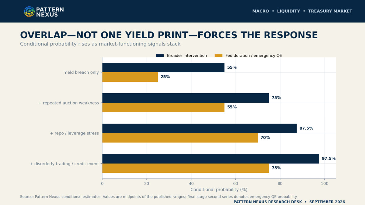
The most important signal is overlap. I am not waiting for one indicator. I am waiting for yield pressure, reserve pressure, funding pressure, and credit pressure to begin reinforcing one another.
That overlap is the switch from forecast to response. Before the switch, the Fed can describe high yields as tight financial conditions doing the work of monetary policy. After the switch, the same yields impair the transmission mechanism the Fed is responsible for preserving. The market price has not necessarily changed much. The institutional meaning of the price has.
11 · LABELS AND MECHANICS
Why the next QE will probably be divided into several programs
The word QE carries too much political and inflationary baggage. In the present environment, an open announcement that the Fed is buying long government bonds to lower borrowing costs would immediately raise questions about fiscal dominance, debt monetization, inflation credibility, and central-bank independence.
The institutional solution is separation.
Reserve-management purchases are separated from monetary-policy easing. Treasury buybacks are separated from Fed asset purchases. Repo is separated from permanent balance-sheet expansion. Portfolio composition is separated from the policy rate. Market-functioning purchases are separated from economic stimulus.
Individually, each statement can be technically true. Together, the programs can reproduce much of the economic machinery of QE.
The names I would expect include:
- Reserve Management Purchases;
- Treasury Market Functioning Operations;
- Liquidity Support Buybacks;
- SOMA Portfolio Composition Adjustments;
- Temporary Duration Liquidity Operations;
- Treasury Market Resilience Purchases;
- Financial Stability Asset Purchases.
I am not predicting the exact branding. I am identifying the institutional logic. The program will be named after the malfunction it claims to repair, not the financial conditions it inevitably changes.
The accounting test is more useful than the press-conference label
I will classify the program through three questions. Did the operation create or preserve reserve balances? Did it remove Treasury or mortgage duration from private balance sheets? Did it establish a state-contingent public buyer that changes the price private markets demand to hold that risk? If one answer is yes, the operation is part of the liquidity architecture. If two or three are yes, the economic substance is moving toward QE regardless of what the statement calls it.
This prevents the analysis from getting trapped in semantics. A temporary repo operation creates reserves but reverses when the loan matures. A Treasury buyback changes the composition and liquidity of government debt but does not create reserves. Operation Twist removes duration without necessarily expanding the net balance sheet. Coupon QE creates reserves and removes duration at the same time. Soft yield-curve control adds a reaction function: private markets know the public buyer becomes larger when the yield or market-functioning signal crosses an internal boundary.
Fiscal dominance will appear as a sequence, not a confession
Fiscal dominance does not require the Federal Reserve to announce that Treasury financing now controls monetary policy. It appears when the cost and market structure of government debt narrow the central bank’s independent choices. The Fed may still set the policy rate according to inflation. But if the Treasury market cannot absorb issuance cleanly at that rate structure, the balance sheet is pulled toward protecting the government collateral layer.
That is why the next program can remain formally separate from deficit finance while functionally making deficit finance easier. Treasury changes issuance and expands buybacks. The Fed protects reserves and repo. The SOMA portfolio shifts toward coupons. Market-functioning purchases compress volatility and term premium. Each action has its own legal and operational explanation. The combined result is a public balance sheet carrying more of the risk the private market rejected.
They do not need to call it QE for it to create reserves, absorb duration, support collateral values, suppress volatility, and lower the private sector’s required return.
12 · WHAT THE SYSTEM IS PROTECTING
This is larger than the Treasury market
The Treasury market is the base collateral layer beneath the system. Stress there does not remain there.
Housing
Mortgage pricing is tied to longer Treasury yields and mortgage spreads, not the federal-funds rate alone. A Fed that holds the overnight rate steady while allowing the 10-year to remain near 5% is still delivering severe restraint to housing. Turnover, refinancing, affordability, construction finance, brokerage activity, and household mobility all remain trapped.
The damage compounds through volume, not only price. Owners with older low-rate mortgages stay in place. Potential sellers do not list because replacing the loan destroys the monthly payment. Builders buy down rates or narrow margins. Buyers qualify for less house. Renovation, furniture, moving, appraisal, title, brokerage, and local tax activity all slow around the frozen transaction. The long end can therefore weaken a large economic network without causing a headline housing-price crash.
The federal interest bill
High long rates compound into fiscal cost as debt rolls over. CBO’s 2026 baseline already projected a $1.9 trillion deficit for fiscal 2026 and net interest outlays near $1 trillion, rising to $2.1 trillion by 2036.[11] A persistent 5% long end increases the amount of future revenue consumed by interest and expands the issuance needed to service the issuance.
This is the fiscal feedback loop behind the duration thesis: higher yields raise interest expense; higher interest expense widens future deficits; wider deficits require more issuance; more issuance requires more balance-sheet capacity; and a saturated balance sheet demands a higher yield. The loop can be interrupted by lower inflation, stronger real growth, fiscal consolidation, shorter issuance, private demand, or public-sector absorption. The current policy mix is leaning most heavily on shorter issuance and public liquidity management.
Banks and insurers
Higher yields reduce the market value of existing fixed-rate assets. Banks may be well capitalized in regulatory terms and still face economic losses, deposit competition, or reduced lending capacity. Insurers and other long-duration institutions carry their own liquidity and valuation mismatch.
The distinction between realized and unrealized losses matters until liquidity forces the issue. A bank can hold a bond to maturity and avoid recognizing the market loss through earnings. But deposits can leave, collateral haircuts can change, or the bank can need cash before maturity. The accounting treatment does not create liquidity. It only determines when the economic loss becomes visible.
Leveraged Treasury trades
Hedge funds can hold enormous Treasury exposure through repo-funded basis trades. The trade can look stable until volatility rises, margins change, or repo terms tighten. Then a small price move creates forced balance-sheet contraction in the deepest market in the world. The Fed’s own July minutes identified near-record hedge-fund leverage and record repo and prime-brokerage borrowing.[6]
AI and infrastructure
The AI buildout is not only an equity narrative. It is data centers, power plants, grids, cooling, chips, transformers, land, construction, and long-lived financed assets. High real duration raises the hurdle rate for that entire physical system. Large firms can survive longer because they have cash, equity, and access. Suppliers, regional developers, utilities, and leveraged projects cannot absorb the same rate indefinitely.
Private credit and regional banks
The July minutes reported rising redemption requests at business development companies, slowing private-credit activity, and growing debt financing of AI capital spending through nonbank investors and regional banks.[6] This creates a bridge between duration stress and the capital boom. If the asset valuations supporting the boom reprice while financing costs remain high, the strongest part of the barbell can become the transmission mechanism into the weakest.
Stablecoins and the front-end collateral machine
Stablecoins and tokenized Treasury products create structural demand for bills and other short government instruments. That is useful for Treasury financing and supports the short end. It also reinforces the maturity split. The newest dollar rails want liquid, short, transparent collateral that can be redeemed quickly. They do not naturally absorb twenty or thirty years of duration.
This means the same collateral evolution that makes bill financing easier can leave the long end more dependent on traditional real-money buyers, foreign institutions, dealers, and leveraged trades. The liquidity machine grows while its preferred maturity becomes shorter. That is not a contradiction. It is one of the structural reasons phase one can succeed while phase two becomes necessary.
The global dollar and foreign Treasury demand
Long Treasuries are not funded inside a closed U.S. system. Foreign reserve managers, banks, insurers, pensions, exporters, sovereign funds, and hedged private investors all participate. Their decision depends on the yield, the dollar, the cost of currency hedging, domestic bond alternatives, regulatory treatment, and confidence in Treasury-market depth.
A strong dollar can increase global demand for dollar liquidity while simultaneously making Treasury ownership more expensive or volatile for an investor whose liabilities sit in another currency. If foreign buyers shorten maturity, hedge more aggressively, or reduce marginal demand, the dealer system has to carry more of the auction. That is one route by which a U.S. fiscal problem becomes a global dollar-funding problem and returns to the Fed through repo, swap lines, or the FIMA repo facility.
The Fed will not intervene merely to make bondholders happy. It will intervene if the Treasury market begins impairing the collateral, funding, and credit machinery attached to it.
13 · CALL AUDIT
What landed, what missed, and what the evidence now requires
The balance-sheet expansion call landed. QT ended in December 2025. Reserve-management purchases began. Treasury holdings rose. The Fed openly adopted the mechanism needed to keep reserves ample. That was the structural core of the QE 2026 thesis.[5][13]
The intermediate steps also arrived in the sequence laid out across the earlier work. The Reverse Repo Trap identified the RRP reservoir and the bill rotation beneath the headline balance sheet.[28] Repo Is Back identified recurring funding operations as the failure mode to watch rather than waiting for a recession headline.[27] Why the Fed Will Try to Keep QE Small argued that the first response would be technical, limited, and divided across tools—and that the market would force expansion if the initial amount failed to stabilize the binding constraint.[26]
The current evidence confirms the first half of that architecture. The Fed kept the initial program small and concentrated in bills. Treasury carried more of the long-end response through buybacks. Repo stress receded. The balance sheet expanded without a public surrender on inflation. That is precisely why the next test is so clean: if long yields continue higher while repo and auctions deteriorate again, the minimal program will have reached its limit.
The expectation that the 10-year would fall much lower did not land. The long end remained high and then moved higher. The miss came from underweighting the persistence of fiscal supply, real capital demand, energy and geopolitical shocks, and the degree to which the Fed could support bills without supporting duration.
The current update does not move the goalposts by pretending bill purchases were the same as full QE. They were not. It divides the original call into two separate phases:
- Reserve-layer expansion: confirmed.
- Duration-layer intervention: not confirmed, but rising in probability.
This is why the current forecast is more useful than simply repeating “QE is coming.” The system has already selected one form of QE-like support. We now have to identify the condition under which that form becomes insufficient.
Treasury’s decision to double long-end buybacks and the FOMC’s discussion of maturity composition are not proof that coupon QE is imminent. They are evidence that both sides of the public balance sheet are building tools around the exact pressure point identified in the framework.[6][8]
14 · INVALIDATION
What would lower the intervention probability
The call weakens materially if the duration problem resolves without public balance-sheet absorption.
I would reduce the six-to-twelve-month probability of a larger program below 35% if the following conditions develop together:
- the 10-year falls and holds below approximately 4.25%;
- the real 10-year falls toward or below 2.00% to 2.10%;
- the 30-year falls below roughly 4.75%;
- inflation decelerates enough to reopen conventional rate cuts;
- Treasury auctions remain consistently strong without rising dealer absorption;
- reserves remain near or above $3 trillion through the late-October TGA peak;
- repo remains orderly and SRF use remains negligible;
- private-credit redemptions, regional-bank exposure, mortgage stress, and credit spreads stabilize;
- Treasury’s expanded buybacks improve liquidity without requiring Fed involvement.
A broad productivity acceleration could also absorb high real rates more cleanly than I expect. If AI investment spreads into wages, suppliers, output, tax revenue, and real household income fast enough, the economy may grow into part of the duration burden rather than forcing immediate monetary absorption.
That is the low-probability clean route. It exists. It is simply not the highest-probability route in the present data.
15 · PATTERN NEXUS LENS
The intervention will appear first as maintenance, then as necessity
Most people are still asking whether the Fed is hawkish or dovish. That is too small a frame for the system now operating.
The Fed can be hawkish on inflation and supportive of reserves. Treasury can issue more debt and simultaneously buy old debt back. The government can increase bill supply while trying to protect the 10-year and 30-year sectors. Stablecoins can create structural Treasury demand while concentrating that demand at the shortest maturities. AI can produce real growth and real inflation pressure at the same time. Households can remain fragile while capital markets remain strong.
These are not contradictions. They are layers.
The LCPI identified the liquidity turn because liquidity returned to the system. The long end identified the routing failure because that liquidity did not remove enough duration. The August CPI report identified the policy constraint because the Fed cannot simply cut until the long end surrenders. Treasury’s buybacks identified the first public response because the pressure has already reached the part of the curve the government cannot ignore.
This leaves a narrow set of paths.
Either inflation and real yields fall cleanly, allowing conventional rate relief to do the work, or the public balance sheet has to absorb more of the duration burden. That absorption can occur through Treasury issuance changes, larger buybacks, reserve-management purchases, repo facilities, maturity transformation, targeted coupon purchases, or full QE.
The names will be different because the politics require different names. The mechanism will remain familiar.
The expanded charts make the full system visible at once. The 10-year and 30-year are directly beneath the stress thresholds. Real yields show that the pressure is not only inflation compensation. The Fed’s portfolio chart shows that almost all of the Treasury expansion occurred in bills. LCI-PCA shows a positive base liquidity regime, while the four-pipe chart shows the TGA acting as the live drain. The reserves/TGA chart identifies late October as the next plumbing test. The repo chart shows that funding is calm today but has already demonstrated how quickly it can cross the threshold. The probability charts show why those observations produce 70% for a larger architecture but only 40% to 45% for direct coupon buying right now.
That difference is not hesitation. It is the structure of the forecast. The broader architecture can expand through Treasury, bills, reserve management, repo, regulation, and maturity changes without requiring full QE. Direct Fed duration purchases become the dominant branch only after the market proves those lower-cost tools cannot carry the load.
My final probability is 70% that the QE-like architecture expands materially within six to twelve months, 40% to 45% that the Fed itself moves into meaningful coupon-duration purchases, and more than 85% conditional on a sustained 10-year above 5%, a 30-year above 5.5%, and visible auction or funding dysfunction.
The highest-probability window begins in late October, builds through year-end, and extends into the first half of 2027.
The Fed fixed the plumbing. If the long end keeps rising, it will have to fix the price and distribution of duration next.
FAQ
Key questions about QE 2026 phase two
Has QE already restarted?
Officially, the Fed calls the program reserve-management purchases, not QE. Mechanically, the Federal Reserve’s Treasury holdings and reserves expanded after QT ended, but the purchases were concentrated in bills and short maturities. I treat that as phase one of the QE-like architecture, not as confirmation of long-duration QE.
Why did bill purchases not lower the 10-year and 30-year?
Bills carry almost no duration risk. Buying them adds reserves and supports short-term rate control, but it does not remove the real-rate and term-premium exposure embedded in long coupon securities. Private investors and dealers still have to absorb that duration.
What is the current probability of a larger program?
My estimate is 70% over the next six to twelve months for a material expansion of the broader QE-like architecture and 40% to 45% for direct Fed coupon-duration purchases. The probability rises above 85% if the yield thresholds are breached alongside auction, repo, leverage, or credit dysfunction.
Could the Fed raise rates and expand the balance sheet at the same time?
Yes. The Fed can use the policy rate to signal its inflation stance while using asset purchases or repo operations to maintain reserves and market functioning. The tools affect different layers even though they interact through overall financial conditions.
What would the program most likely be called?
The most likely labels are reserve management, Treasury-market functioning, portfolio-composition adjustment, liquidity support, market resilience, or financial-stability purchases. The name will probably describe the malfunction being repaired rather than call the action quantitative easing.
Would Treasury buybacks alone solve the problem?
They can improve liquidity and shorten the effective maturity of public financing if long coupons are replaced with bills. But Treasury cannot create reserves or absorb duration at the scale of the Federal Reserve. Buybacks are the first defense and may delay Fed action; they cannot guarantee it will never be needed.
What is the most likely timing?
The September FOMC is more likely to prepare the architecture than launch duration QE. The first major window is late October through early November as the TGA peaks and bill issuance rises. December and the first half of 2027 are the stronger windows if long rates and funding pressure persist.
Is hard yield-curve control likely?
Not immediately. A soft, unnamed reaction function is much more likely than a public yield cap. The Fed can buy more aggressively when yields, volatility, auctions, or market depth breach internal limits without promising to defend one exact rate forever.
What would invalidate the forecast?
A sustained fall in nominal and real long yields, orderly auctions, reserves remaining ample through the TGA rebuild, stable repo, improving credit, and inflation cooling enough to permit conventional rate cuts would materially reduce the probability of duration intervention.
Sources
Data, policy documents, and prior Pattern Nexus framework
- [1] U.S. Department of the Treasury, Daily Treasury Par Yield Curve Rates, September 10, 2026.
- [2] U.S. Department of the Treasury, Daily Treasury Par Real Yield Curve Rates, September 10, 2026.
- [3] U.S. Bureau of Labor Statistics, Consumer Price Index—August 2026, September 11, 2026.
- [4] Board of Governors of the Federal Reserve System, H.4.1 Factors Affecting Reserve Balances, September 10, 2026.
- [5] Federal Reserve Bank of New York, Treasury Securities Operational Details, accessed September 11, 2026.
- [6] Board of Governors of the Federal Reserve System, Minutes of the Federal Open Market Committee, July 28–29, 2026, released August 19, 2026.
- [7] U.S. Department of the Treasury, Quarterly Refunding Statement, August 5, 2026.
- [8] U.S. Department of the Treasury, Treasury Announces Increased Sizes of Nominal Long-End Liquidity Support Buybacks Beginning September 9, August 19, 2026.
- [9] Board of Governors of the Federal Reserve System, FOMC Meeting Calendars and Information, accessed September 11, 2026.
- [10] Federal Reserve Bank of New York, Roberto Perli, Reflections on the Early Days of Reserve Management Purchases, March 26, 2026.
- [11] Congressional Budget Office, The Budget and Economic Outlook: 2026 to 2036, February 11, 2026.
- [12] Pattern Nexus, Two Economies, One Balance Sheet: The Unstable Barbell of 2026, September 10, 2026.
- [13] Pattern Nexus, QT Ends, Liquidity Returns: Why 2026 Is Almost Certainly the Next Balance-Sheet Expansion Cycle, November 25, 2025.
- [14] Pattern Nexus, Hard Assets Follow Liquidity, Not Inflation—A Full Data Reconstruction, 2025.
- [15] Pattern Nexus, Hard Assets Follow Liquidity: The LCI Framework White Paper, January 2026.
- [16] Pattern Nexus, The Plumbing Update: The Four Pipes and the Liquidity Composite, February 27, 2026.
- [17] Pattern Nexus, The Calm Before the Liquidity Storm: QE 2026 and the Digital Evolution of Money, October 17, 2025.
- [18] Pattern Nexus, The Treasury Just Drew Its Line in the Sand—And It’s at the 10-Year, November 5, 2025.
- [19] Pattern Nexus, Fiscal Dominance and the Sticky Term Premium: Why Long Rates Stay High, October 18, 2025.
- [20] Pattern Nexus, The Gravity Zone: How the 10-Year Treasury Revealed the Real Neutral Rate, November 18, 2025.
- [21] Pattern Nexus, Pattern Nexus Macro Archive and Public Record, 2025–2026, updated 2026.
- [22] Federal Reserve Bank of St. Louis, FRED economic data: WALCL, WTREGEN, RRPONTSYD, M2SL, WRESBAL, DGS10, DGS30, DFII10, DFII30, SOFR, and IORB, retrieved September 11, 2026.
- [23] Board of Governors of the Federal Reserve System, Decomposing Hedge Funds’ U.S. Treasury Exposures, June 22, 2026.
- [24] Federal Reserve Bank of New York, Recent Developments in Treasury Market Liquidity and Funding Markets, May 9, 2025.
- [25] Board of Governors of the Federal Reserve System, Financial Stability Report: Leverage in the Financial Sector, May 2026.
- [26] Pattern Nexus, Why the Fed Will Try to Keep QE Small—and Why It Won’t Work in 2026, December 27, 2025.
- [27] Pattern Nexus, Repo Is Back: Late-2025 Looks Like Late-2019, December 29, 2025.
- [28] Pattern Nexus, The Reverse Repo Trap: How the Fed Quietly Controls Liquidity and Markets, October 31, 2025.
Editorial note: This article separates current observations, official program labels, Pattern Nexus interpretation, scenario probabilities, estimated future program design, and the prior public call record. Reserve-management purchases are not described as officially announced QE. This is research and educational analysis, not individualized investment advice.
Pattern Nexus analyzes systems upstream of the public narrative: incentives, chokepoints, liquidity, infrastructure, energy, balance sheets, collateral, and control structures.
Christopher Grenke / Pattern Nexus Research Desk · September 11, 2026
What's Your Reaction?
 Like
0
Like
0
 Dislike
0
Dislike
0
 Love
0
Love
0
 Funny
0
Funny
0
 Wow
0
Wow
0
 Sad
0
Sad
0
 Angry
0
Angry
0

Nexus (Christopher)
Founder of Pattern Nexus. I research markets, macro, geopolitics, AI, history, ancient systems, and the patterns most people overlook. I’m also building Market Radar, a trading scanner designed to read pressure, risk, confirmation, and setup quality before ch…
Related research

The New American Crypto Order: How Trump’s Executive Actions, Treasury Strategy, and Federal Reserve Alignment Are Rewiring the Dollar System
The United States has quietly shifted from restricting crypto to absorbing it. Trump’s Strategic Bitcoin Reserve, the Digital Asset Stockpi…
🧭 IMF Warns Global Debt Could Exceed 100% of GDP by 2029
The IMF’s latest Fiscal Monitor warns that world public debt could climb beyond 100 percent of GDP by 2029 — a threshold unseen since the a…
Why the Fed Will Try to Keep QE Small — and Why It Won’t Work in 2026
The Fed will try to keep QE “light” in 2026 to protect inflation credibility and avoid backlash. But modern market plumbing is nonlinear: u…

Fed Chair Odds as a Term-Premium Signal: Warsh Takes the Lead
Prediction markets are repricing Trump’s Fed chair pick toward Kevin Warsh. In the Pattern Nexus framework, this is not “personality politi…
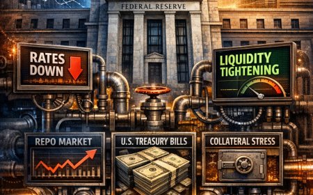
Warsh’s Fed and the Balance-Sheet War: Why “Rates Down” Can Still Mean “Liquidity Tight”
A Pattern Nexus systems read on the incoming Fed regime debate: floor vs corridor, repo backstops, Treasury supply, and why the balance she…
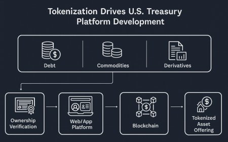
The Dollar Isn’t Collapsing — It’s Evolving
The dollar isn’t dying — it’s upgrading. The U.S. converts liabilities into globally demanded collateral (Treasuries), backstopped by the w…
Comments (0)
Security Check
Please complete the captcha to verify you are human.