

Treasury’s Long-Bond Relief Could Bring a Faster Refinancing Cycle
Treasury’s larger long-end buybacks can improve trading today. PN follows the actual cash payments, September maturity data, and replacement-financing choices to test whether that relief could bring …
Jump to a section
Treasury has expanded its support for older long-dated bonds. Four October operations accepted $6 billion of face value each, following the August decision to increase long-end buyback capacity. The market benefit can be real: investors gain a scheduled opportunity to sell securities that trade less readily than the newest issues.[1][2][3][4][5][9]
The financing trade-off depends on the debt issued alongside those purchases. Replacing long fixed-rate obligations with shorter funding would bring some future financing decisions forward. Falling rates would then reach the budget sooner; persistently high or rising rates would do the same. The operation results do not identify a dedicated bill auction funding each buyback.
The existing calendar makes that trade-off worth watching. At September 30, $10.6402 trillion of marketable interest-bearing debt matured within one year, against $31.8312 trillion outstanding. Average maturity was still 70 months. A long average and a large near-term refinancing queue can coexist.[6]
My working hypothesis is that the more useful signal will come from the combination of buybacks, net issuance by maturity, and the rate-reset calendar. Larger purchases alone cannot establish that Treasury has accelerated the refinancing cycle. The November financing announcements will provide the next policy evidence.
Which long-dated obligations does Treasury retire?
Face value and the current funding requirement differ.
The overall issuance mix determines the new obligations.
Maturity and interest-rate reset set the future exposure.
01 · BUYBACKS AND REFINANCING
The long end has a larger buyer
On August 19, Treasury said the maximum size of liquidity-support buybacks in the nominal 10-to-20-year and 20-to-30-year sectors would increase from $2 billion to at least $4 billion per operation. The change began September 9 and applied through the refunding quarter ending November 4. Treasury cited strong participation and high-quality offers in those sectors.[1]
By October, the final operation results showed a $6 billion maximum and $6 billion accepted at each of four long-end operations. The October 1 and October 15 purchases covered the 10-to-20-year range; October 8 and October 27 covered the 20-to-30-year range. Together they retired $24 billion of par value.[2][3][4][5]
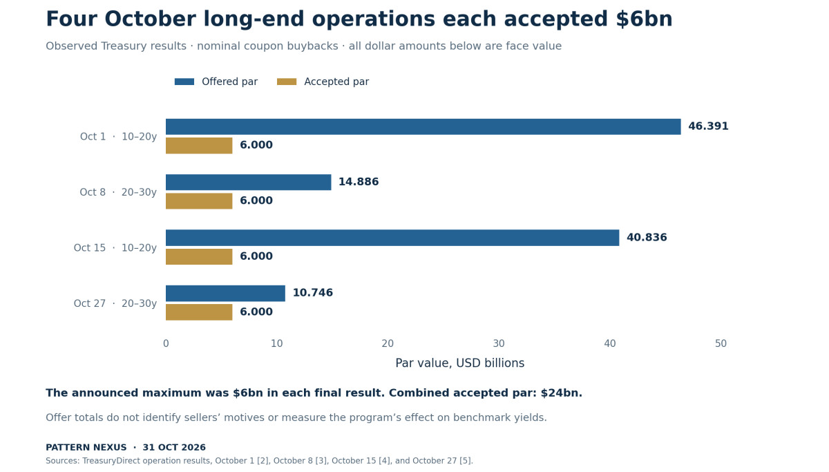
The offer totals varied considerably. Participants offered $46.391 billion on October 1 and $40.836 billion on October 15, compared with $14.886 billion on October 8 and $10.746 billion on October 27. Those amounts describe securities submitted for sale at participants’ chosen prices. They do not reveal how urgently each holder needed cash or the market value of every eligible security.[2][3][4][5]
That limits what an oversubscribed operation can tell us. A large offer book may reflect an attractive opportunity to sell, relative-value positions, inventory management, or other motives. Treasury evaluates offers against prevailing prices and relative value. The accepted amount is evidence of an executed purchase, rather than a direct measure of distress.[9]
PN’s August article, “Treasury Turns Long-Bond Buybacks Into a Yield-Control Test,” interpreted the expanded program as a potential pressure valve for the long end. That was an analytical interpretation of its possible market role. The official announcement established liquidity support and larger operation sizes; it did not announce a benchmark yield target.[1][13]
The October results now let us examine the securities being removed and the cash needed to remove them. Those details lead directly to the replacement-funding question.
02 · BUYBACKS AND REFINANCING
What the operation buys
Treasury describes liquidity-support buybacks as a regular opportunity to sell off-the-run securities: older issues that have been displaced by newer benchmarks. Cash-management buybacks have a separate purpose, including smoothing seasonal cash balances and bill issuance. The distinction matters when comparing programs that retire very different maturities.[9]
A scheduled buyer can make an older bond easier to hold. A dealer considering a customer’s sale can take the next operation into account when deciding how much inventory to absorb and at what price. An investor can consider the operation when planning a portfolio adjustment. These are potential channels through which regular purchases could improve market functioning; the published results do not quantify their effects.
The benefit need not appear as a sustained fall in the 10-year or 30-year benchmark yield. It could appear in the cost of trading an eligible older security, the price difference between related issues, or the inventory a dealer is willing to carry. Benchmark yields also respond to inflation expectations, the prospective policy rate, issuance, and investors’ compensation for holding duration.
That makes the evaluation more demanding than checking whether yields fell on announcement day. A useful liquidity program can coexist with higher benchmark yields. A favorable yield move can also occur without proving that the program improved trading conditions.
The debt-management question begins after that market benefit is acknowledged. A government that removes a long-dated obligation must account for the cash paid now and the financing obligations that remain afterward.
03 · BUYBACKS AND REFINANCING
Six billion of bonds is not six billion in cash
The October 27 operation accepted $6 billion of par value across six bonds maturing between May 2048 and May 2051. Their coupons ranged from 1.875% to 3.125%. Treasury’s result gives the accepted par amount and weighted average accepted price for each security.[5]
Multiplying each accepted amount by its published price per $100 of par produces an estimated clean payment of $3.84367 billion. The aggregate price is approximately $64.061 per $100 of face value. This is PN arithmetic using prices rounded by Treasury to three decimal places. Accrued interest must be added to reach the settlement amount.[5][14]
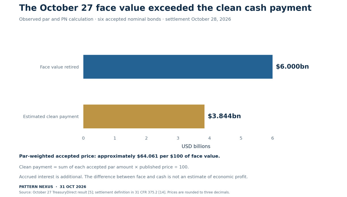
The difference is central to the financing analysis. The operation retired $6 billion of future principal obligations, but the clean cash payment was about $3.844 billion. Describing it as a $6 billion cash purchase would overstate the immediate funding requirement. Treating the difference as an immediate economic gain would overstate the benefit.
Those older bonds promised relatively small coupons over a long period. A market discount adjusts the price investors will pay for those remaining cash flows. Treasury pays the market price to cancel them, including the future principal payment. The discount has an economic reason.
For a deliberately simplified illustration, suppose new debt issued at par financed exactly the clean purchase price. Treasury would retire $6 billion of old face value and issue about $3.844 billion of new face value. That would reduce face value in this isolated comparison. The calculation excludes accrued interest and assumes an issuance price and financing match that the actual operation results do not establish.
An economic assessment also needs the interest and maturity terms of the replacement, the cash-flow timing, and a consistent valuation basis. A smaller face amount can carry a higher coupon rate. A lower coupon bill can carry a much earlier refinancing date. Face value, current cash payment, and future financing exposure answer different questions.
04 · BUYBACKS AND REFINANCING
The funding pool sets the replacement
Treasury’s buyback authority allows the use of proceeds from debt sales and other money in the general fund. Its borrowing-estimate footnote says buybacks are not expected to significantly affect privately held net marketable borrowing because new issuance replaces securities bought back.[8][9]
That explains the broad funding relationship. It does not assign a particular new bill, note, or bond to a particular repurchase. Treasury finances its combined cash requirements. Tax receipts, spending, debt maturities, cash-balance decisions, and buybacks all enter that funding problem.
The marginal comparison therefore requires a counterfactual: what mix would Treasury have issued without the additional buybacks? If the extra cash requirement is met through bills while planned long-term issuance stays unchanged, the combined policy can remove long fixed-rate obligations and add shorter obligations. That would bring the relevant replacement financing back to market sooner.
If Treasury instead expands longer fixed-rate issuance, the maturity effect could be smaller or reverse. If available cash covers an operation temporarily, the immediate transaction still does not settle the eventual financing choice. The timing of cash use and replenishment matters.
August’s refunding statement said Treasury expected nominal coupon and floating-rate-note auction sizes to remain unchanged for at least the next several quarters. It also described bills and cash-management bills as tools for seasonal and unexpected financing needs. That makes the bill channel plausible, but it does not prove which securities financed October’s repurchases.[7]
I would test the hypothesis across several financing periods. A recurring pattern of long-end retirement alongside greater reliance on short funding would be more informative than a single operation. The program’s size must also be compared with the much larger outstanding debt stock.
05 · BUYBACKS AND REFINANCING
A long average, a near-term queue
Treasury’s fourth-quarter data workbook reports $31.8312 trillion of marketable interest-bearing debt outstanding at the end of September. The maturity distribution places $10.6402 trillion within one year and $11.0628 trillion between one and five years. The remaining buckets extend beyond five years.[6]
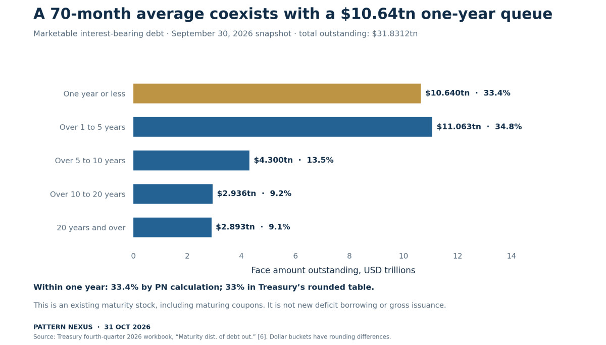
The within-one-year amount represents approximately 33.4% of the reported stock, calculated from the dollar amounts. Treasury’s rounded percentage is 33%. Its separate cumulative maturity table reports 46% maturing within 24 months and 55% within 36 months. Those windows overlap; they should not be added together.[6]
Average maturity was 70 months in September, compared with 71 in June. That one-month difference does not establish that the expanded long-end buybacks caused a material shortening of the whole portfolio. Issuance, ordinary redemptions, the passage of time, and other operations all affect the average.[6]
The four October operations in Figure 1 retired face value equal to approximately 0.075% of September’s reported outstanding stock. This comparison is only a scale check: October operations occur after the September snapshot, and other buybacks are outside the four-operation sample. It shows why a claim that these purchases have transformed the entire debt structure would outrun the evidence.
The near-term amount deserves attention for a different reason. Financing conditions encountered during the next year will reach a substantial existing maturity queue. New deficits add funding needs; refinancing replaces obligations already outstanding. Both appear at auctions, but they have different meanings for the change in debt.
The one-year bucket includes maturing coupon securities as well as bills. It is also a stock measured on one date. A short bill that matures and is reissued several times during the following year creates repeated auction volume, even though the initial stock counted it once. That is how a large gross issuance calendar can sit beside a smaller outstanding amount.
06 · BUYBACKS AND REFINANCING
The 85.9% number needs its denominator
The same Treasury workbook reports that bills accounted for 85.9% of actual marketable issuance in fiscal 2026’s fourth quarter, which ran from July through September. A headline built around that number alone would invite readers to confuse repeated issuance with the composition of the debt stock.[6]
Three measures should be kept in view:
| Measure | Latest reported observation | What it describes |
|---|---|---|
| Bills as a share of actual marketable issuance | 85.9%, July–September 2026 | Gross issuance composition; short instruments can turn over repeatedly |
| Net bill borrowing | $427.481 billion, July–September 2026 | The workbook’s bill contribution to net marketable borrowing |
| Marketable debt maturing within one year | $10.6402 trillion at September 30 | A maturity bucket covering bills and maturing coupon securities |
The workbook reports $742.342 billion of total net marketable borrowing for that quarter. Dividing the bill contribution by that total gives approximately 57.6%. That is a contribution ratio using this table’s accounting, including its separate negative buyback entry. It is not the percentage of buybacks financed by bills.[6]
The 85.9% and 57.6% figures describe different flows. Neither is the bill share of outstanding debt. Neither, by itself, establishes a deliberate maturity-shortening policy.
For the proposed mechanism, the useful question is whether the incremental financing mix persistently gives rates more opportunities to reset. That requires looking through the repeated turnover in gross auction totals and keeping the cash-balance objective alongside issuance.
07 · BUYBACKS AND REFINANCING
Maturity and rate reset run on different clocks
A maturity date tells us when principal must be repaid or refinanced. It does not always tell us when the interest rate changes. Treasury floating-rate notes make the difference visible: they mature in two years, pay interest quarterly, and reset their index weekly using the latest 13-week bill auction’s highest accepted discount rate. Their spread is fixed for the life of the note.[10]
| Funding form | Principal clock | Interest-rate clock |
|---|---|---|
| Short bill rolled into a new bill | Repayment at each maturity | New financing terms at the next issue |
| Two-year Treasury FRN | Principal due after two years | Index resets weekly; interest is paid quarterly |
| Long fixed-rate nominal bond | Principal due at its stated maturity | Coupon rate remains fixed for that bond |
This creates two ways for current rates to reach future interest costs. Treasury can refinance maturing fixed-rate debt at new terms. It can also pay a changing index on floating-rate debt before principal matures. A debt portfolio with a longer legal maturity can still contain instruments that respond quickly to short rates.
Conversely, a rise in a fixed-rate bond’s market yield changes its trading price without rewriting Treasury’s contractual coupon. New borrowing and refinancing will encounter the new market; an existing fixed coupon continues under its original terms unless the obligation is retired.
The financing dashboard should therefore track maturity and rate-reset exposure separately. Treasury’s workbook includes a weighted-average-next-rate-reset sheet alongside the maturity tables. The series have different scopes and should be read with their definitions, rather than substituted casually for one another.[6]
The hypothesis in this article is about shortening the government’s financing decisions at the margin. Replacing long fixed-rate debt with bills and replacing it with FRNs would create different principal calendars, even if both made interest costs more responsive to near-term rates.
08 · BUYBACKS AND REFINANCING
The cost of choosing a shorter clock
Consider an illustrative $100 billion funding balance. Assume one option locks a 5% annual rate through the second year. The other starts at the same rate but fully refinances at the start of year two. Let the replacement rate be 3%, 5%, or 7%.
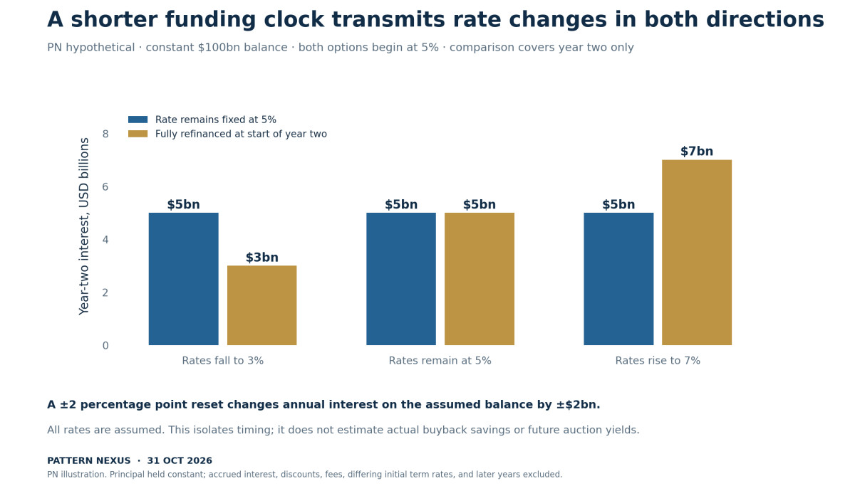
The locked-rate option costs $5 billion in year-two interest in every case. The refinancing option costs $3 billion, $5 billion, or $7 billion. A two-percentage-point move changes the annual interest cost on this assumed balance by $2 billion. All amounts and rates are hypothetical.
The shorter choice provides faster savings when rates fall. It also passes higher rates through faster. It gives up some certainty about future terms in exchange for flexibility and the possibility of lower cost. The eventual result depends on the rate path and the terms available when financing is arranged.
This illustration holds the funding balance constant and isolates one year of interest. It excludes issuance discounts, transaction costs, accrued interest, changes in principal needs, and differences in the original rates available at different maturities. It does not model the October 27 buyback or forecast an auction yield.
Actual debt management is more complex because new financing arrives continuously and obligations mature on different dates. A diversified maturity schedule spreads exposure across those dates. A concentrated short schedule gives the government more frequent contact with the current rate environment.
That contact can become politically significant before refinancing becomes operationally difficult. Faster interest-cost transmission changes the budget consequences of a prolonged period of high short rates. It does not dictate the Federal Reserve’s policy decision or establish that Treasury will struggle to complete an auction.
09 · BUYBACKS AND REFINANCING
Why the discount is not a fiscal windfall
The October 27 bonds carried about $159.885 million of annual contractual coupons in aggregate, calculated from the accepted par amounts and coupon rates. Retiring them removes those future coupons and their principal obligations. The cash raised to finance the purchase has its own cost.[5]
Comparing the old 2.66475% weighted coupon with a new borrowing rate would still be incomplete. The old coupon applies to $6 billion of face value. Replacement financing for the purchase would relate to the cash requirement, including accrued interest, and could have a different face amount and maturity. The two percentages would sit on different bases.
The market discount also incorporates the timing of principal. Cancelling a dollar due decades from now is different from cancelling a dollar due next month. A proper cost comparison puts the old and new cash flows on a consistent basis and considers the risk of future refinancing.
It is possible for a repurchase to reduce reported face value and improve market functioning while increasing exposure to near-term refinancing rates. It is also possible for the financing terms to make that choice attractive. Those outcomes can coexist because the measures capture different effects.
The strongest claim the available results support is concrete: Treasury retired specified long-dated cash flows at specified market prices. The net lifetime saving or cost requires replacement-funding assumptions and a rate path. The face-value discount alone cannot supply either.
10 · BUYBACKS AND REFINANCING
The reserve flow needs both sides
Treasury purchases are conducted through the New York Fed acting as fiscal agent. That operating role does not turn a Treasury-funded repurchase into a Federal Reserve portfolio purchase. The fiscal funding source remains relevant even when the transaction uses Federal Reserve infrastructure.[9]
When Treasury pays out of its account at the Fed and the proceeds reach a bank deposit, the payment can increase bank reserves, holding other flows constant. Financing that payment through debt issuance can move cash in the other direction. Tax receipts, government spending, and the identity and funding source of security buyers also affect the reserve result.
The gross buyback amount therefore cannot establish a lasting reserve injection. A full assessment needs the Treasury cash-account path and the financing flows around settlement. The $6 billion par amount from October 27 is an especially poor substitute because it exceeds even the clean cash payment.
This connects with PN’s broader liquidity framework: follow the balance-sheet entries and their timing. For this article, the additional step is to follow the obligation created when Treasury replenishes the cash it used. The settlement effect and the future refinancing effect belong to different points on the same calendar.
11 · BUYBACKS AND REFINANCING
The budget adds a reason to watch timing
The September Monthly Treasury Statement reports approximately $1.052 trillion of net interest outlays for fiscal 2026. Its separate gross interest line for Treasury debt securities is $1.359953 trillion. The measures have different coverage; the gross figure should not be substituted for the budget’s net-interest function.[12]
Those totals establish the scale of the existing interest burden. They do not measure the cost of the expanded buybacks. Much of the year preceded the August announcement, and the budget includes obligations far beyond this program.
The timing argument is prospective. When more funding resets quickly, a change in market rates can reach interest outlays sooner. When funding remains fixed for longer, more of that adjustment is delayed. The effect also depends on how much debt is exposed and on the direction of rates.
A small operation does not explain a trillion-dollar annual total. Repeated financing choices can still influence how rapidly a large portfolio responds over time. That is the scale at which this mechanism becomes useful: as a debt-management path to monitor, rather than a dramatic attribution to one month’s purchases.
12 · BUYBACKS AND REFINANCING
What November can actually tell us
As of this article’s October 31 cutoff, the next borrowing estimate is scheduled for November 2 and the next quarterly refunding announcement for November 4. Their contents are still future information. The last August estimate projected $628 billion of privately held net marketable borrowing in October–December, assuming an $850 billion end-December cash balance.[8][15]
A revision to that borrowing estimate will need to be read with its cash assumptions. A larger projected cash buffer can increase borrowing without an equivalent increase in the underlying deficit. A reduction can work in the opposite direction. Comparing headline borrowing numbers without the opening and closing cash balances can misidentify the driver.
Treasury’s November dealer agenda already supplies a useful set of questions. It asks about the effects of larger buybacks on liquidity, dealer intermediation, and client participation, as well as prospective coupon and FRN issuance and structural demand. These are consultation questions, not announced policy decisions or published dealer answers.[11]
I would look for whether the next documents extend the larger long-end operations, alter their frequency or limits, and explain any associated financing changes. A bigger purchase schedule without a change in funding composition would tell a different story from a sustained expansion supported by shorter incremental borrowing.
The auction schedule also matters operationally. More frequent financing creates more settlement dates that must fit around receipts, spending, and market capacity. The relevant evidence is the adopted calendar and its results, rather than every scheduling possibility raised during consultation.
13 · BUYBACKS AND REFINANCING
Three paths through the same program
The program can evolve in several directions. The purchase size alone will not distinguish them.
| Conditional path | Evidence to look for | Financing implication |
|---|---|---|
| Liquidity improves with little change in the funding clock | Better trading measures in eligible issues; stable maturity and reset exposure | Market-functioning benefits with a limited portfolio-level timing change |
| Long-end support expands alongside shorter incremental financing | Repeated long-end retirement, greater net short issuance after cash adjustments, faster reset exposure | More frequent contact with the rate environment; gains if rates fall, costs if they rise |
| Replacement financing extends or preserves fixed-rate exposure | Longer fixed-rate issuance offsets the obligations retired | A smaller acceleration, or a different maturity result from the proposed hypothesis |
These paths describe mechanisms to test. They are not assigned probabilities. The first could leave the central refinancing hypothesis largely unsupported while still making the liquidity program useful. The second would strengthen it. The third would require the article’s expected transmission to be revised.
Market conditions can also change the trade-off. Investors may value short collateral differently from long duration. A functioning long-end market can help Treasury issue longer securities on better terms. If liquidity improvements support that longer issuance, some of the apparent tension between today’s relief and tomorrow’s calendar could diminish.
That feedback is a reason to observe both sides of debt management. Buybacks affect the stock available to trade. New issuance determines the obligations Treasury adds. Their combined effect can differ from the impression created by either announcement in isolation.
14 · BUYBACKS AND REFINANCING
The refinancing dashboard
I would keep six items together when updating this thesis:
- Executed purchases: accepted par, estimated cash paid, coupons, maturity dates, and the concentration of purchases across individual securities.
- Incremental financing: net issuance by instrument and maturity, with buybacks and ordinary redemptions identified rather than hidden inside gross auction totals.
- Cash assumptions: opening and closing Treasury cash, seasonal receipts, and the stated reason for borrowing revisions.
- Principal calendar: the shares maturing within one, two, and three years, alongside average maturity and the dollar amounts involved.
- Rate-reset exposure: floating-rate financing and the timing at which changing rates can enter interest costs before principal repayment.
- Market-functioning results: transaction costs, depth, and relative pricing of eligible securities, with benchmark yields treated as a broader outcome.
The dashboard deliberately combines benefits and costs. Stronger liquidity with stable refinancing exposure would be a favorable result. Faster rate transmission with falling rates could also lower financing costs. A less comfortable combination would be shorter exposure, persistent high rates, and limited improvement in trading conditions.
No single threshold here establishes a funding crisis. The purpose is to detect a changing transmission channel early enough to evaluate it. Repeated observations matter more than a large number in one auction or a brief yield reaction.
PATTERN NEXUS VIEW
The Pattern Nexus view
The feature I would watch is the migration of exposure across time. Treasury can remove a difficult-to-trade long obligation today while making a new financing decision sooner, depending on what it issues alongside that purchase. The market may notice the first effect immediately. The budget encounters the second over the replacement instrument’s life.
October’s results establish that the long-end intervention has grown beyond the old $2 billion operation limit. September’s debt data establish a substantial existing refinancing queue. August’s financing guidance establishes that bills remain an adjustment tool. Those facts make the mechanism plausible; they do not establish a matched transfer from each long bond into bills.[1][2][3][4][5][6][7]
The useful next question is how much certainty Treasury is retaining about future funding terms as it improves today’s market. If the answer is less, the rate path becomes more consequential sooner. If longer fixed-rate issuance preserves that certainty, the hypothesis weakens. The next financing decisions should be judged against that observable choice.
READER QUESTIONS
Frequently asked questions
Has Treasury announced a yield cap?
The August announcement set larger liquidity-support operation limits for specified long-end sectors. It did not announce a target yield or a commitment to buy whatever amount would defend one. PN’s earlier yield-control framing was an interpretation of the possible market role. Purchase results alone cannot establish that a benchmark yield has been controlled.[1][13]
Do the October results prove that bills financed the purchases?
They report the securities accepted and their prices. They do not identify a matched financing auction. Treasury funds combined cash requirements through its general cash and issuance program. Testing a shift toward short funding requires the broader issuance mix, cash assumptions, and a comparison with what would otherwise have been issued.[5][8][9]
Did Treasury pay $6 billion on October 27?
It accepted $6 billion of face value. PN’s calculation from the six accepted securities and published prices gives approximately $3.84367 billion before accrued interest. Prices are rounded, so this is an estimate of the clean payment rather than the exact settlement cash. The distinction matters for both the funding requirement and any claimed reduction in face value.[5][14]
Is one-third of the debt coming due the same as one-third in bills?
The September table’s one-year maturity bucket includes bills and coupon securities approaching maturity. It is a remaining-maturity measure. It also differs from gross issuance, which can count repeated refinancing of short instruments during the period. The workbook’s outstanding stock is marketable interest-bearing debt, rather than gross national debt.[6]
Would shorter financing always raise interest costs?
The result depends on rates and the terms chosen. Shorter financing can transmit falling rates into costs sooner and can transmit higher rates sooner. Figure 4 isolates that symmetry using assumed rates and a constant funding balance. It does not estimate the program’s actual lifetime saving, cost, or optimal maturity mix.
Can rates reset before a Treasury security matures?
Yes. A Treasury FRN matures in two years, but its index resets weekly and interest is paid quarterly. The spread established when the note is first offered remains fixed. That means principal maturity, index reset, and cash payment have different schedules. A fixed-rate nominal bond’s coupon does not change merely because its market yield moves.[10]
What would weaken the article’s hypothesis?
Evidence that replacement financing preserves or extends fixed-rate exposure would weaken it. So would stable portfolio-level reset exposure despite larger buybacks. Better liquidity with only a small maturity effect would support a narrower market-functioning interpretation. The hypothesis should change with the issuance and maturity evidence; it does not follow automatically from a rising purchase limit.
METHOD AND EVIDENCE
Method and evidence
Research cutoff: October 31, 2026. Operation amounts and accepted securities come from TreasuryDirect’s four dated October result PDFs. The September debt stock, maturity distribution, fiscal-quarter issuance breakdown, and net borrowing figures come from Treasury’s fourth-quarter 2026 workbook. Fiscal 2026 interest figures come from the September Monthly Treasury Statement.
PN calculations include par-weighted accepted prices, estimated clean purchase payments, retired annual contractual coupons, ratios calculated from workbook dollar amounts, and the hypothetical interest comparison. The clean-payment calculation sums accepted par multiplied by published price divided by 100; it excludes accrued interest and inherits price rounding.
The four-operation sample is not the whole buyback program. The September stock predates the October transactions. Rounded maturity buckets may not sum exactly to the reported total. Cumulative maturity windows overlap. No auction-level replacement financing, causal yield effect, forced-selling motive, or lifetime fiscal profit is inferred from the operation results.
The article’s central proposition is a conditional debt-management mechanism. The source record establishes the transactions and financing context; future issuance and rate outcomes determine whether the proposed acceleration occurs.
SOURCES
Research and Data Sources
Official Treasury results, financing statements, and debt data establish the observed record. PN calculations and the conditional refinancing mechanism are identified separately.
- U.S. Department of the Treasury. Treasury Announces Increase in Size of Liquidity Support Buybacks for Longer-Dated Nominal Coupon Securities. August 19, 2026. Increase from $2bn to at least $4bn for the two long-end buckets, effective September 9 through the quarter ending November 4. No announced yield peg.
- TreasuryDirect. Treasury Debt Buyback Operation Results — October 1. October 1, 2026; settlement October 2. 10–20-year nominal operation; accepted par, offers, maximum, and security-level prices.
- TreasuryDirect. Treasury Debt Buyback Operation Results — October 8. October 8, 2026; settlement October 9. 20–30-year nominal operation; amounts are par rather than cash.
- TreasuryDirect. Treasury Debt Buyback Operation Results — October 15. October 15, 2026; settlement October 16. 10–20-year nominal operation; final maximum and accepted amount are both $6bn.
- TreasuryDirect. Treasury Debt Buyback Operation Results — October 27. October 27, 2026; settlement October 28. Six accepted CUSIPs; rounded published prices support PN estimates of clean payment and retired contractual coupons.
- U.S. Department of the Treasury. Fourth-Quarter 2026 Quarterly Refunding Data. Released October 16, 2026; debt snapshot September 30. Workbook sheets: Maturity dist. of debt out.; % debt maturing next 12-36 mths; % Breakdown of qrtly iss; Net marketable borrowing; Avg. mat. of debt outstanding; WANRR. Fiscal Q4 is July–September.
- U.S. Department of the Treasury. Quarterly Refunding Statement. August 5, 2026. Coupon and FRN issuance guidance and use of bills for financing adjustments. Its initial buyback plan preceded the August 19 increase.
- U.S. Department of the Treasury. Treasury Announces Marketable Borrowing Estimates. August 3, 2026. October–December estimate of $628bn with $850bn end-cash assumption; buyback financing footnote. Estimate, not realized borrowing.
- TreasuryDirect. FAQs about Treasury Securities Buybacks. Current FAQ, accessed October 31, 2026. Authority, purposes, retirement, fiscal-agent process, offer evaluation, and publication of prices.
- TreasuryDirect. Floating Rate Notes. Current terms, accessed October 31, 2026. Two-year maturity, weekly index reset, quarterly payment, and fixed spread.
- U.S. Department of the Treasury. November 2026 Dealer Agenda. October 2026 consultation; refunding announcement scheduled November 4. Questions on buyback effects, financing composition, demand, and scheduling. Questions do not establish adopted policy.
- Bureau of the Fiscal Service. Monthly Treasury Statement — September 2026. Fiscal 2026 year-end report, published October 2026. Net interest approximately $1.052tn in the functional presentation; gross Treasury-security interest $1,359,953m in Table 3. Different coverage.
- Pattern Nexus / AI Nexus. Treasury Turns Long-Bond Buybacks Into a Yield-Control Test. August 22, 2026. Prior PN interpretation of the expanded program. Not the source for a formal yield target or proof of refinancing changes.
- U.S. Department of the Treasury / Federal Register, Government Publishing Office. Marketable Treasury Securities Redemption Operations — final rule. March 30, 2026; 91 FR 15540–15543; effective March 30. 31 CFR 375.2 defines settlement amount as accepted par times price, plus accrued interest. Official GPO text used; historical proposed rules excluded.
- U.S. Department of the Treasury. Most Recent Quarterly Refunding Documents. Accessed October 31, 2026. Official release schedule: next borrowing estimate November 2, next policy release November 4; workbook and dealer agenda released October 16.
Public research on Treasury market structure and the financing calendar. This article is available free, without a premium or registration gate.
Article overview
Treasury’s larger long-end buybacks can improve trading today. PN follows the actual cash payments, September maturity data, and replacement-financing choices to test whether that relief could bring future interest-rate exposure forward.
What's Your Reaction?
 Like
0
 Dislike
0
 Love
0
 Funny
0
 Wow
0
 Sad
0
 Angry
0

Nexus (Christopher)
Founder of Pattern Nexus. I research markets, macro, geopolitics, AI, history, ancient systems, and the patterns most people overlook. I’m also building Market Radar, a trading scanner designed to read pressure, risk, confirmation, and setup quality before ch…
Related research
Ample Reserves, Uneven Liquidity
Aggregate reserves can support rate control while funding conditions differ by institution. PN examines October research, overnight-rate di…
5 shared topics, 1 shared asset, same research avenue.
The Treasury Market Is Changing Its Gatekeepers
Treasury clearing deadlines are approaching. PN examines who gains from netting and cross-margining, how access and funding terms shape the…
4 shared topics, 1 shared asset, same research avenue.
The Interest Trap: Borrowing a Trillion Dollars to Service the Debt
The United States finished fiscal 2026 with a $1.992 trillion deficit. Net interest accounted for $1.052 trillion of it. I break down the b…
5 shared topics, same research avenue.
Fed Just Hiked Into a 5% 10-Year: Why the Next Liquidity Cycle May Arrive Faster
The Federal Reserve just raised the federal-funds target to 3.75%–4.00% while the 10-year Treasury closed at 5.01%, the 30-year at 5.35%, a…
8 shared topics, 1 shared asset, same research avenue.
QE 2026, Phase Two: When the Long End Forces Duration Control
The Fed already ended QT and expanded Treasury holdings through bill-focused reserve-management purchases, but that repaired the reserve la…
4 shared topics, 1 shared asset.
August CPI Just Activated the Fed’s One-Hike Option—and Deepened the Long-End Trap
August CPI rose 0.4% on the month and 3.4% from a year earlier, while core CPI rose a hotter-than-expected 0.3% even as its annual rate eas…
5 shared topics, 1 shared asset, same research avenue.
Two Economies, One Balance Sheet: The Unstable Barbell of 2026
Reserve support has returned, but real long rates, fiscal supply, and an AI-energy capital wave are splitting the U.S. economy between capi…
5 shared topics, 2 shared assets, same research avenue.
Treasury Turns Long-Bond Buybacks Into a Yield-Control Test
Treasury said it will raise maximum liquidity-support buybacks in the 10-to-20-year and 20-to-30-year nominal coupon sectors from $2 billio…
5 shared topics, same research avenue.
Comments (0)
Security Check
Please complete the captcha to verify you are human.