
The Capital Ladder: Where $100 to $1 Trillion Places You in the Global and American Wealth System
A deep Pattern Nexus regression and data analysis mapping where net worth levels from $100 to $1 trillion place an individual within the global and American wealth distributions. The research separates actual net worth from liquidity, accessible credit, gross capital control, leverage, and daily capital-producing capacity. Where do you actually sit within the global wealth system—and how does that position change when we measure not only what you own, but how much capital you can access? This research maps wealth levels from $100, $500, and $1,000 through $1 million, $1 billion, $100 billion, and the theoretical $1 trillion threshold. Global and American wealth distributions are analyzed separately using regression models, percentile estimates, Federal Reserve household data, international wealth-distribution research, and 17 original charts and visualizations. The analysis distinguishes net worth from liquid wealth, available credit, collateral-backed borrowing capacity, and gross capital controlled. It then models how productive leverage can accelerate wealth growth, how destructive leverage can erase equity, and how much daily capital output different levels of wealth may generate. Net worth measures ownership. Liquidity measures deployability. Credit measures reach. Leverage amplifies the result. Capital efficiency determines whether that amplification creates wealth or debt.

The global wealth distribution is so compressed that approximately $29,200 places an adult at the entrance to the global top half, while roughly $265,600 enters the global top 10%, $2 million enters the global top 1%, and $1 billion reaches approximately the top one-in-a-million adults.
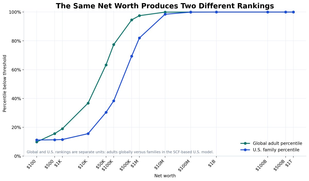
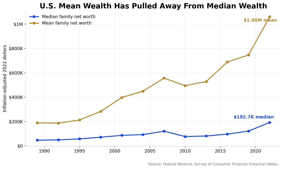
The American distribution is different. The 2022 Survey of Consumer Finances placed median U.S. family net worth at $192,700 and mean family net worth at $1.059 million. A million dollars therefore ranks extremely high globally—about the 97.50th percentile in this model—but only around the 82.01st percentile among U.S. families.
The regression work finds that inflation-adjusted U.S. mean family wealth rose at an estimated 5.21% annual trend from 1989 through 2022, versus 3.29% for median family wealth. The aggregate balance sheet compounded materially faster than the typical balance sheet.
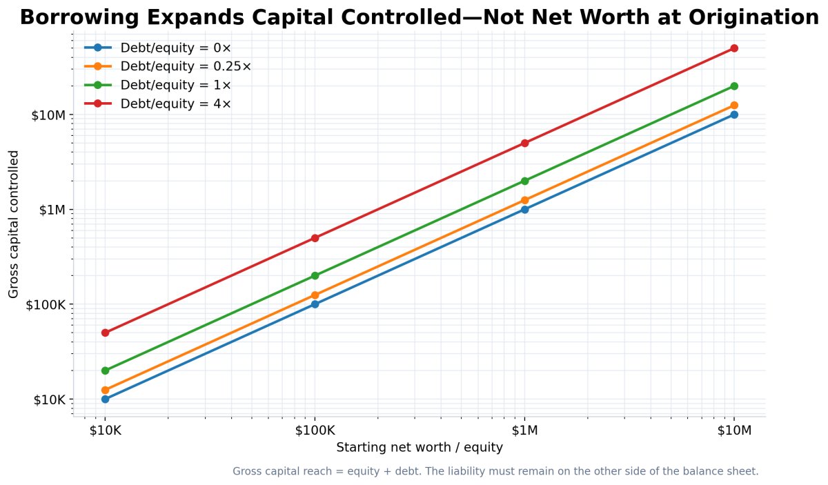
Capital access is not net worth. Borrowing $400,000 against $100,000 of equity gives a person control of a $500,000 gross asset base, but they still begin with $100,000 of net worth. The leverage only creates wealth if the after-cost return on the deployed assets exceeds interest, fees, taxes, losses, and depreciation.
Pattern Nexus conclusion: wealth is not one ladder. It is at least four ladders—ownership, liquidity, capital access, and capital efficiency. Two people with identical net worth can have completely different probabilities of moving upward because one owns deployable, financeable assets and the other owns trapped or depreciating equity.
This report combines the World Inequality Report 2026 global threshold ladder, the Federal Reserve’s 2022 Survey of Consumer Finances historical and cross-sectional tables, the Fed’s Distributional Financial Accounts framework, the World Bank Global Findex 2025, UBS Global Wealth Report 2026 context, and extreme-tail billionaire rank data.
It then builds separate global-adult and U.S.-family percentile models, runs time-series and cross-sectional regressions, compares Pareto and curved extreme-tail fits, creates a leverage spread model, calculates daily capital-output capacity, and publishes every requested wealth level from $100 through $1 trillion.
The global model and American model are never merged into one false distribution. Adults are not households. PPP wealth is not market-exchange-rate wealth. Survey wealth is not a real-time billionaire list. Borrowing capacity is not equity. Every one of those boundaries is maintained.
The world does not sort people only by how much wealth they currently own. It sorts them by how much of that wealth is liquid, how much income it can produce, how much outside capital it can attract, what collateral it can support, and whether the person can compound a positive spread between asset returns and capital costs.
That is why a person with $50,000 in cash, strong income, low liabilities, and access to productive financing may possess greater upward mobility than a person with $100,000 trapped in an illiquid or deteriorating asset. The second person is wealthier on paper. The first may control more deployable capital.
But leverage does not magically move a person up the wealth distribution. At the moment a loan is created, assets and liabilities rise together. Net worth is unchanged. Only future performance changes equity.
The actual mechanism is simple:
Ending equity = (starting equity + debt) × (1 + asset return)
              − debt × (1 + financing cost)
              − fees, taxes, losses and depreciation
Positive spread compounds ownership. Negative spread destroys ownership. The same leverage that allows someone to cross several tiers of capital control can erase their original tier of net worth.
- The Four Wealth Hierarchies
- Data Architecture and Measurement Rules
- The Global Wealth Distribution
- The Complete $100-to-$1-Trillion Ladder
- Global Tail Regression
- The American Wealth Distribution
- U.S. Wealth Growth Regression, 1989–2022
- What American Balance Sheets Are Made Of
- Liquidity and Capital Access
- The Capital Access Model
- Leverage: Productive, Neutral, and Destructive
- Daily Net Worth and Daily Capital Output
- Housing, Race, Age, and Structural Position
- The Billionaire and Trillion-Dollar Tail
- Regression Results and What They Prove
- Uncertainty, Limitations, and What Not to Claim
- The Final Pattern Nexus Read
- Sources
The Four Wealth Hierarchies
The normal public conversation collapses every financial dimension into one number called net worth. That number matters. It is the cleanest measure of existing ownership. But it is not the entire capital system.
Hierarchy One: Net Worth
Net worth = total assets − total liabilities
This is the equity already owned. It answers the question: if every asset were valued correctly and every liability were paid, what remains?
Hierarchy Two: Liquid and Deployable Capital
A dollar in a transaction account is not economically identical to a dollar of equity in a private business, a primary residence, a pension, restricted stock, an undeveloped parcel, or a collectible. All may count toward net worth. They do not have the same transaction speed, collateral quality, price certainty, tax cost, or ability to fund the next opportunity.
Hierarchy Three: Accessible Capital
Accessible capital includes available credit, secured borrowing capacity, business financing, margin capacity, mortgage capacity, partner capital, and other funds a person or entity can plausibly command. It is not wealth. It is the external balance sheet available to the person.
Hierarchy Four: Capital Efficiency
Capital access matters only when the borrower can deploy capital at a return exceeding its all-in cost. A person with low-cost, long-duration financing and productive assets occupies a completely different system from a person using 29% revolving credit to fund consumption.
Data Architecture and Measurement Rules
This analysis uses several datasets because no single source can answer every question. The datasets measure different units, use different valuation frames, and operate at different frequencies.
Global Distribution: Adults in a PPP Framework
The World Inequality Report 2026 estimates an adult population of approximately 5.6 billion in 2025 and provides threshold, group-average, group-share, and long-run growth estimates from the bottom half through the top one-in-100-million. The global ladder is therefore modeled per adult.
The WIR comparison uses a purchasing-power framework. That is useful for comparing real economic position across countries, but it is not identical to the market-dollar valuation used in UBS wealth reports or Forbes rankings.
United States: Families in the Survey of Consumer Finances
The Federal Reserve’s 2022 Survey of Consumer Finances is the latest completed SCF. It measures U.S. families and includes balance sheets, pensions, income, and demographic characteristics. The public data contain five implicates because missing observations are multiply imputed. This article uses the Fed’s published historical public tables for core estimates rather than pretending a simple unweighted CSV calculation is equivalent to official SCF estimation.
Current U.S. Calibration: Distributional Financial Accounts
The DFA provides quarterly estimates from 1989 through the latest quarter. It integrates the SCF’s distributional information with the Financial Accounts’ aggregate balance sheets, reconciling concepts and interpolating or forecasting between triennial SCF surveys. The DFA is used as the current structural frame, not to overwrite the detailed 2022 SCF family tables.
Capital Access: Financial Inclusion, Not Fictional Credit Limits
The Global Findex is the only worldwide demand-side financial inclusion survey. It reports account ownership, savings, borrowing behavior, digital access, and emergency funding access. It does not provide globally comparable individual credit limits. Therefore this report does not fabricate a universal regression that claims to predict how much every person on Earth can borrow.
Instead, capital access is modeled as a separate capacity layer using observable proxies: liquid assets, collateral, income stability, debt-service capacity, business ownership, formal account access, and the cost and maturity of capital.
The Global Wealth Distribution
The global distribution is not merely unequal. It is structurally compressed across billions of adults and then stretched almost vertically in the final fractions of one percent.
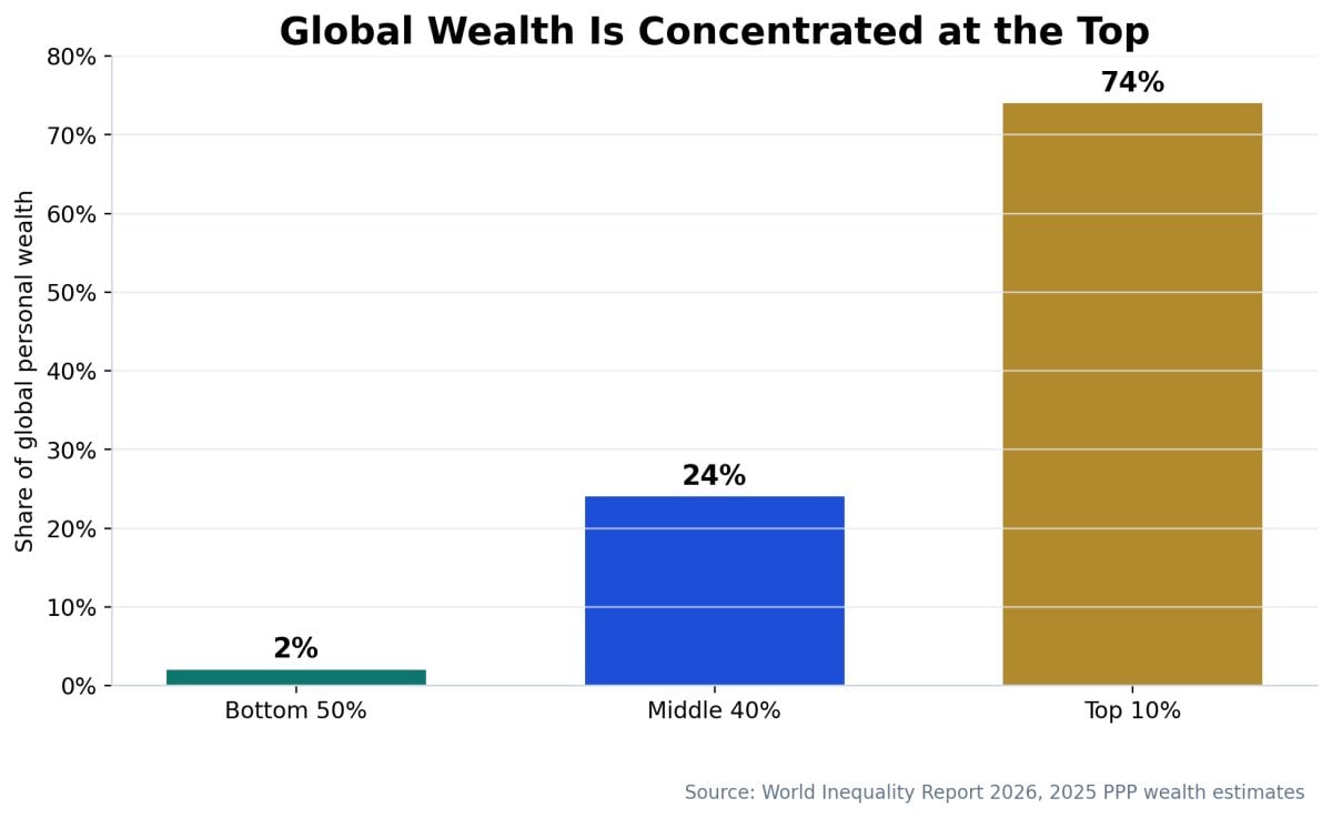
The WIR 2026 estimates that the bottom 50% of adults owns about 2% of global wealth, the middle 40% owns about 24%, and the top 10% owns approximately 74%. The executive summary rounds the top share to three-quarters and the middle share to 23%, but the full ladder figure provides the more detailed 2/24/74 split used here.
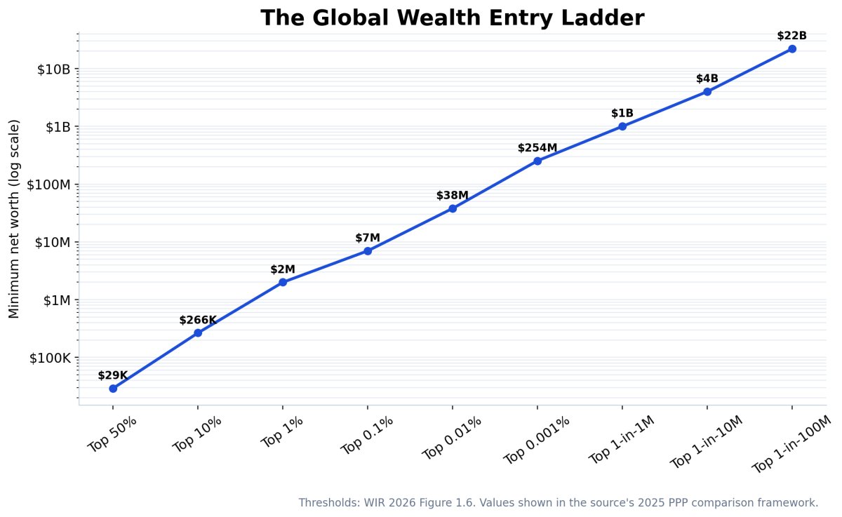
Those shares become more intuitive when translated into entry thresholds:
- $29,200 enters the global top half.
- $265,600 enters the global top 10%.
- $2 million enters the global top 1%.
- $7 million enters the top 0.1%.
- $38 million enters the top 0.01%.
- $254 million enters the top 0.001%.
- $1 billion reaches approximately the top one-in-a-million.
- $4 billion reaches approximately the top one-in-10-million.
- $22 billion reaches approximately the top one-in-100-million.
The average adult in the bottom half owns only about $6,500 in the WIR framework. The average member of the global top 10% owns about $1 million. The average member of the global top 1% owns about $6 million. The average member of the top one-in-100-million owns roughly $53 billion.
This is why average global wealth can be a deceptive statistic. The mean is pulled upward by the same extreme tail that produces the distribution’s political, financial, and institutional power.
The Growth Rate Is Also Unequal
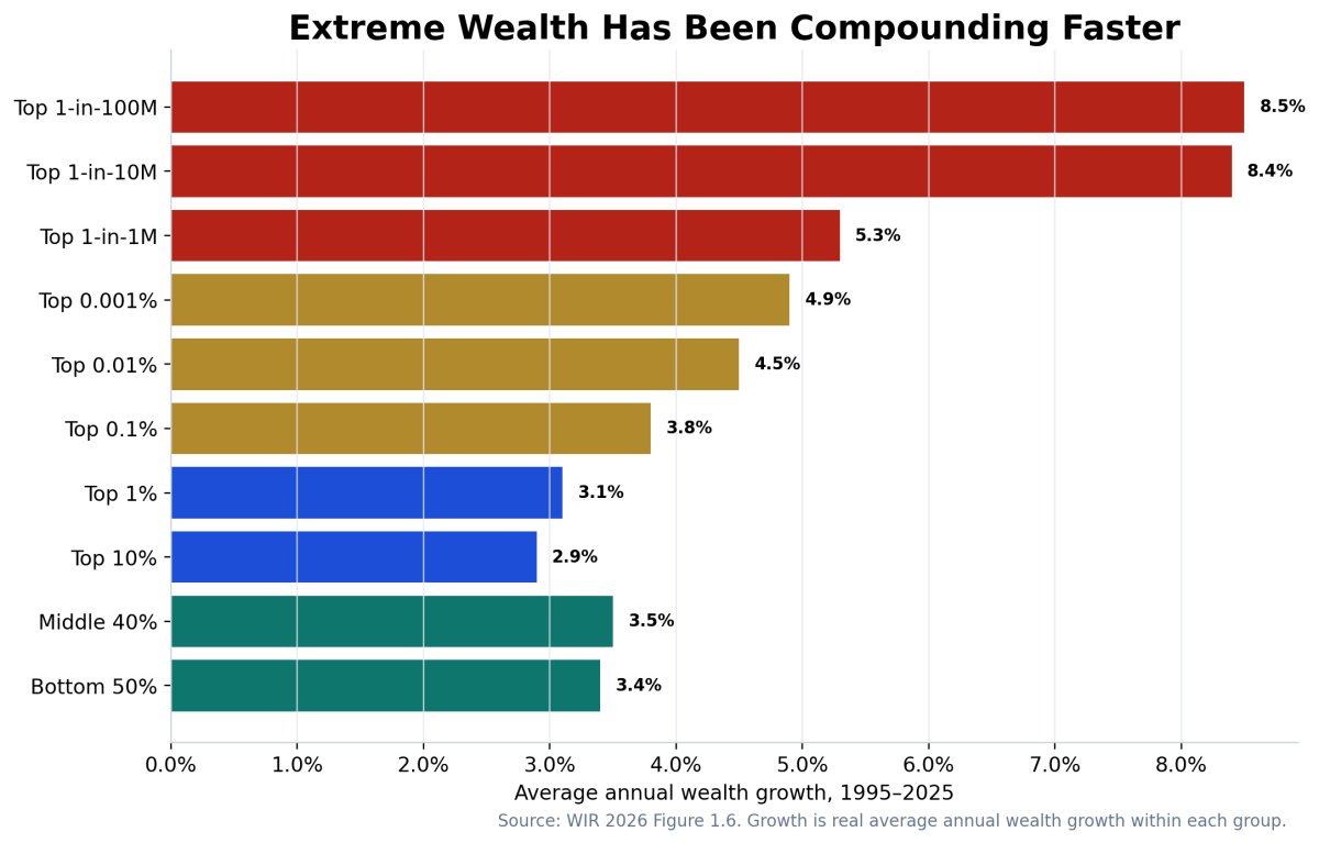
From 1995 through 2025, real wealth growth in the bottom half averaged approximately 3.4% annually. The top one-in-10-million and top one-in-100-million groups compounded around 8.4% and 8.5% annually. A five-percentage-point annual spread sustained for 30 years is not a small difference. It is a different compounding universe.
The Complete $100-to-$1-Trillion Ladder
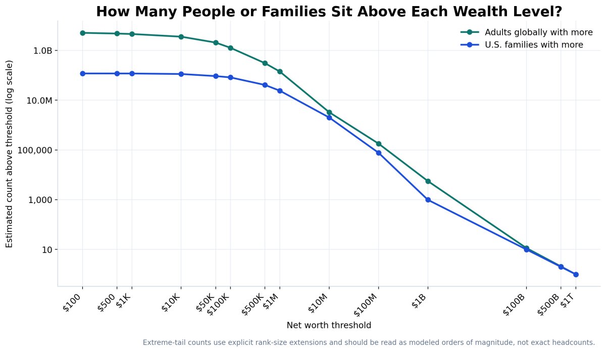
The table below contains every level requested. It shows the modeled global adult percentile, the modeled U.S. family percentile, the number estimated to remain above the threshold, the simple net-worth-per-day scale, theoretical daily capital output at 5%, and capital controlled under two leverage structures.
| Net worth | Net worth ÷ 365 | 5% output/day | Global percentile | Global adults richer | U.S. family percentile | U.S. families richer | Capital controlled at 1× D/E | Capital controlled at 4× D/E |
|---|---|---|---|---|---|---|---|---|
| $100 | $0.27 | $0.01 | 9.84% | 5.05 billion | 11.16% | 117.92 million | $200 | $500 |
| $500 | $1 | $0.07 | 15.60% | 4.73 billion | 11.31% | 117.72 million | $1K | $2.5K |
| $1K | $3 | $0.14 | 19.03% | 4.53 billion | 11.50% | 117.47 million | $2K | $5K |
| $10K | $27 | $1 | 36.79% | 3.54 billion | 15.57% | 112.07 million | $20K | $50K |
| $50K | $137 | $7 | 63.32% | 2.05 billion | 30.35% | 92.45 million | $100K | $250K |
| $100K | $274 | $14 | 77.44% | 1.26 billion | 38.40% | 81.77 million | $200K | $500K |
| $500K | $1.4K | $68 | 94.553% | 305.02 million | 69.35% | 40.69 million | $1M | $2.50M |
| $1M | $2.7K | $137 | 97.498% | 140.10 million | 82.01% | 23.87 million | $2M | $5M |
| $10M | $27.4K | $1.4K | 99.941593% | 3.27 million | 98.489% | 2.01 million | $20M | $50M |
| $100M | $274K | $13.7K | 99.996799% | 179.3 thousand | 99.942061% | 76.9 thousand | $200M | $500M |
| $1B | $2.74M | $137K | 99.999900000% | 5.6 thousand | 99.999254918% | 989 | $2B | $5B |
| $100B | $273.97M | $13.70M | 99.999999797% | 11 | 99.999992494% | 10 | $200B | $500B |
| $500B | $1.37B | $68.49M | 99.999999963% | 2 | 99.999998495% | 2 | $1T | $2.50T |
| $1T | $2.74B | $136.99M | 99.999999982% | <1 | 99.999999247% | <1 | $2T | $5T |
The low-dollar global estimates are modeled rather than directly published threshold points. The WIR gives the bottom-half average of $6,500 and the global top-half entry point of $29,200. A bounded power distribution calibrated to those two values produces a baseline estimate that approximately 36.8% of adults fall below $10,000. UBS separately reports that roughly 41% of adults sit below $10,000 in its market-dollar wealth pyramid. The two frameworks are not identical, but the proximity provides a useful external check.
What the Ladder Says
$100: roughly the 9.84th global percentile and 11.16th U.S. family percentile in the baseline models. This should be read as an order-of-magnitude placement because zero and negative net worth are compressed near the bottom.
$10,000: around the 36.79th global percentile but only the 15.57th U.S. family percentile. The same sum has much greater relative weight globally than inside the American balance-sheet system.
$100,000: approximately the 77.44th global percentile but the 38.40th U.S. family percentile.
$500,000: approximately the 94.55th global percentile and 69.35th U.S. family percentile.
$1 million: approximately the 97.50th global percentile and 82.01st U.S. family percentile.
$10 million: roughly the 99.9416th global percentile and 98.4888th U.S. family percentile.
$100 million: roughly the 99.9968th global percentile and 99.9421st U.S. family percentile.
$1 billion: approximately one-in-a-million globally and around 989 U.S. household-equivalent units above the threshold under the extreme-tail calibration.
$100 billion through $1 trillion: these are rank-space values more than ordinary percentiles. At that scale, reporting “100th percentile” loses meaning. The useful measurement is the expected number of people remaining above the threshold.
Global Tail Regression
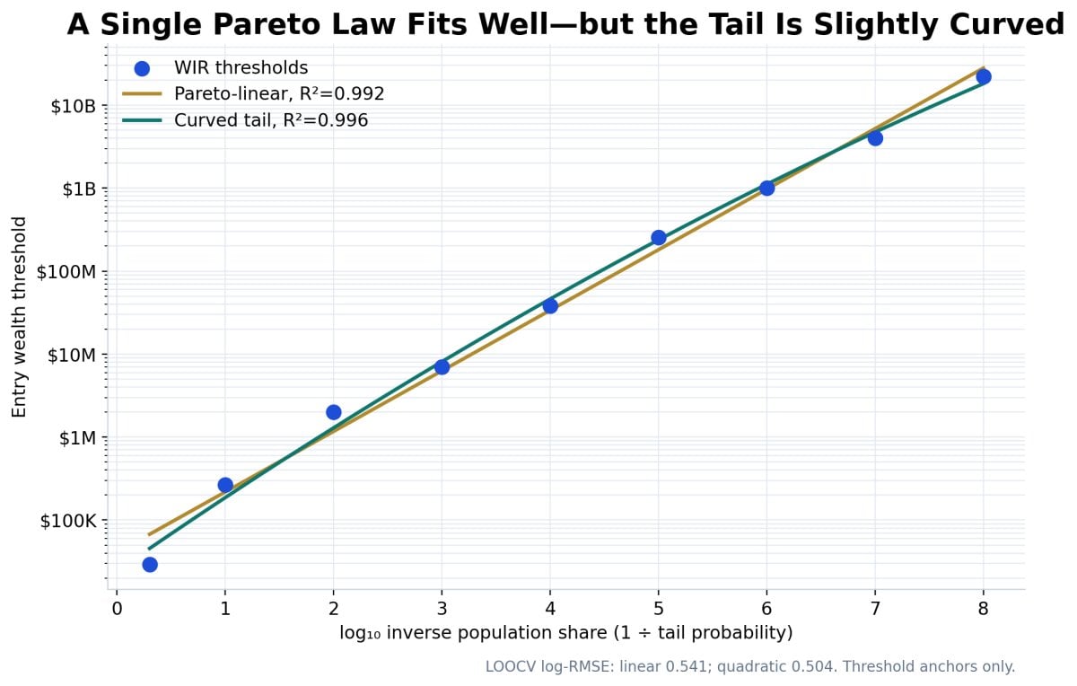
A common mistake is to assume the entire upper wealth distribution follows one perfect Pareto law. Power laws are useful, but they are not magic. The correct question is whether a linear relationship in log threshold versus log inverse-tail probability provides an adequate fit—and whether a curved alternative materially improves it.
Model One: Pareto-Linear Tail
log(wealth threshold) = β₀ + β₁ × log(1 / tail probability) + ε
Across the nine WIR entry thresholds from the global median to the top one-in-100-million, the linear model produces R² = 0.992. The estimated slope is 0.729, implying a Pareto shape parameter near 1.371.
Model Two: Curved Tail
log(wealth threshold) = β₀ + β₁x + β₂x² + ε
where x = log(1 / tail probability)
The quadratic model increases R² to 0.996, lowers AIC from 12.09 to 7.92, and lowers leave-one-out log RMSE from 0.541 to 0.504.
That is evidence of mild curvature, not proof of a universal mathematical law. There are only nine grouped threshold anchors. The result supports using a flexible tail model and uncertainty bands rather than blindly extrapolating one straight line to infinity.
Extreme Rank Extension
Beyond the published $22 billion top one-in-100-million threshold, this article uses an explicit rank-size extension anchored at roughly 56 adults above $22 billion and a one-person $1 trillion boundary. That extension produces estimated counts of about 11 above $100 billion, about two above $500 billion, and about one at $1 trillion.
Those are not precise census counts. They are a transparent way to preserve the requested ladder without pretending a grouped global distribution can identify the exact number of people at continuously changing mark-to-market valuations.
The American Wealth Distribution
The United States must be analyzed separately because the country is much wealthier than the global median and because the SCF’s unit is the family, not the adult.
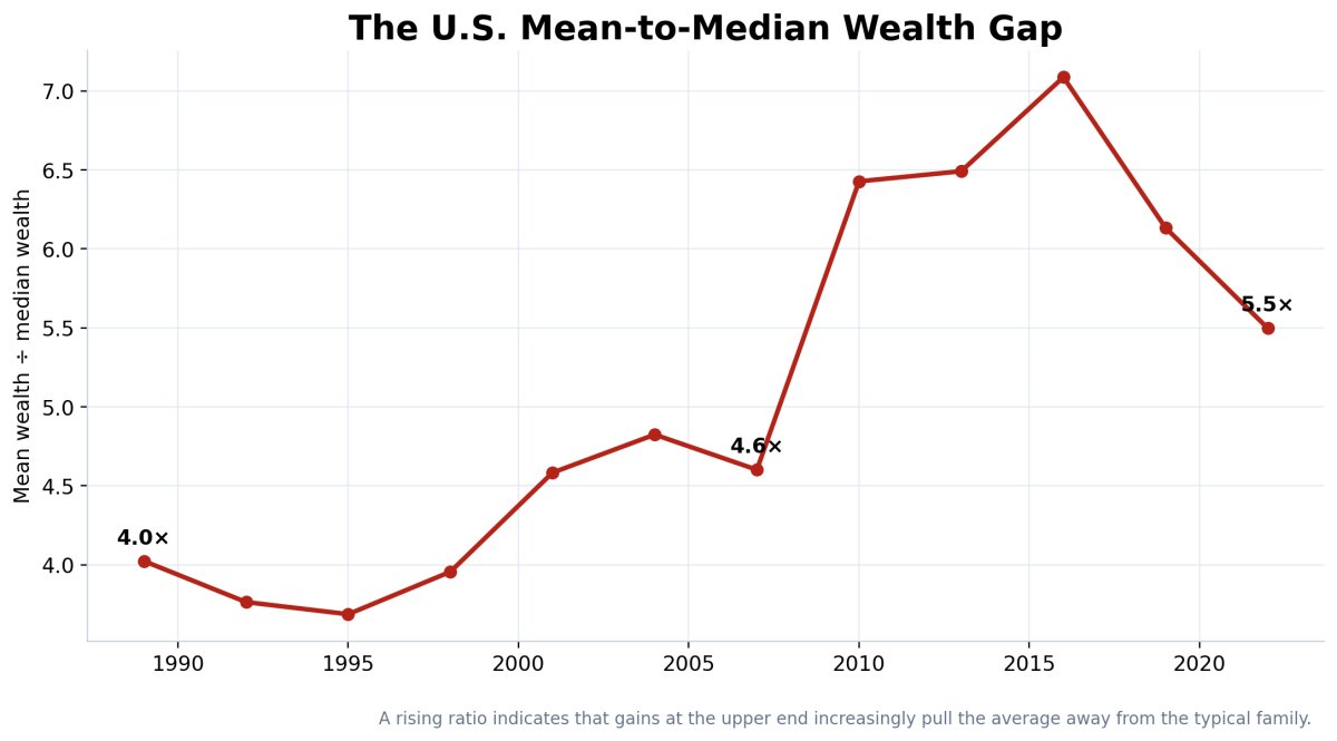
In 2022, median U.S. family net worth was $192,700. Mean family net worth was $1,059,470. The mean was therefore approximately 5.50 times the median.
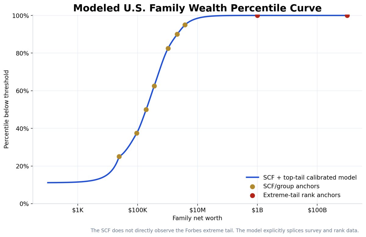
The SCF percentile-group medians provide the middle anchors:
- Bottom 25% group median: $3,470.
- 25th–49.9th percentile group median: $93,400.
- Overall median: $192,700.
- 50th–74.9th percentile group median: $356,900.
- 75th–89.9th percentile group median: $1.036 million.
- Top 10% group median: $3.795 million.
Those are group medians, not group boundaries. This model treats them as approximate quantile anchors at the midpoint of each group and separately uses an external top-10 threshold cross-check near $2.1 million. The extreme tail is then spliced to billionaire rank data rather than pretending the SCF directly observes the Forbes population.
The Bottom Quarter
The bottom-quarter SCF group has a median net worth of about $3,470 and a mean of negative $5,650. To avoid inventing arbitrary low-end thresholds, the model uses a shifted exponential quantile function calibrated to those two facts. It implies a modeled 25th-percentile boundary near $24,100.
That construction places $100 near the 11.16th percentile, $1,000 near the 11.50th percentile, and $10,000 near the 15.57th percentile. These estimates are intentionally marked as modeled because low-end net worth is shaped by negative balances, student debt, medical debt, auto loans, and families with little measurable asset ownership.
U.S. Wealth Growth Regression, 1989–2022
The historical SCF series allows a direct test of whether the average American balance sheet and the typical American balance sheet compounded at the same rate. They did not.
Log Trend Results
Using inflation-adjusted 2022-dollar estimates for all 12 SCF survey years from 1989 through 2022:
- Median family net worth trend: 3.29% annually, R² 0.758.
- Mean family net worth trend: 5.21% annually, R² 0.949.
The 1.92-percentage-point annual trend difference compounds dramatically across 33 years. It does not mean every rich family earned 5.21% and every median family earned 3.29%. It means the aggregate cross-sectional mean rose much faster than the median across the survey history.
The Gap Ratio
The mean-to-median ratio was about 4.0× in 1989. It reached 4.6× in 2007, jumped above 6× after the financial crisis, reached approximately 7.1× in 2016, and stood at 5.5× in 2022.
The fall from the 2016 ratio does not mean concentration disappeared. The absolute mean-minus-median gap expanded from roughly $142,000 in 1989 to approximately $867,000 in 2022. Median wealth rose strongly from 2019 to 2022, reducing the ratio even while the dollar gap widened.
Breakpoint Test
A piecewise log trend with a 2007 breakpoint estimated median growth near 3.72% before 2007 and 2.74% after 2007. Mean growth was approximately 6.07% before the breakpoint and 4.12% after it. But the information criteria barely improved for the mean and worsened for the median. The data do not justify presenting 2007 as one clean permanent regime break.
The better interpretation is that the series contains a housing-and-financial crash, a slow median recovery, and then a large 2019–2022 jump. A single smooth trend is incomplete, but a rigid two-line story is also incomplete.
What American Balance Sheets Are Made Of
Net worth alone does not reveal financial mobility. The composition of the balance sheet determines whether wealth can be deployed, collateralized, diversified, or lost.
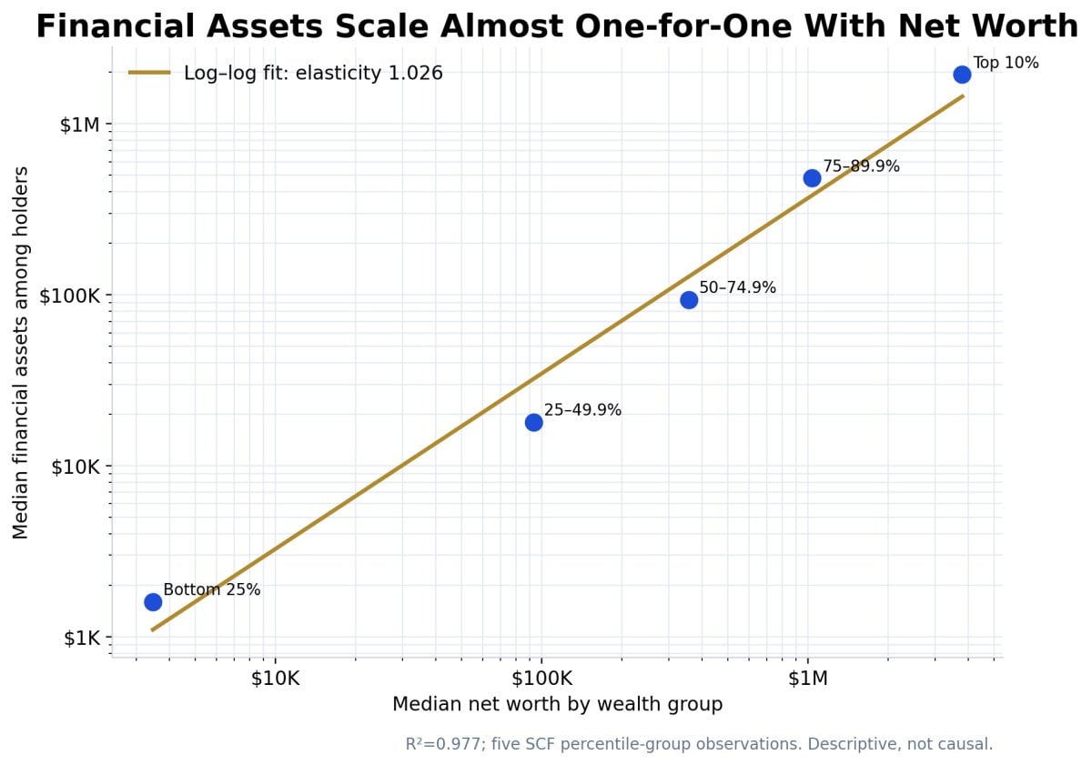
Financial Assets Scale Almost One-for-One
Across the five SCF wealth groups, the regression of median financial assets among holders on median net worth produces an elasticity of approximately 1.026 with R² 0.977. A 1% increase in group median net worth is associated with approximately a 1.03% increase in median financial assets among asset holders.
This is one of the strongest findings in the cross-sectional analysis. Wealthier groups do not simply own more total assets. They own disproportionately scalable financial claims.
Transaction Balances Scale More Slowly
Transaction account balances have an estimated elasticity of 0.693, R² 0.961. Cash-like balances grow with wealth, but not one-for-one. At higher levels, a larger share of the balance sheet shifts into securities, retirement accounts, businesses, real estate, private assets, and other claims.
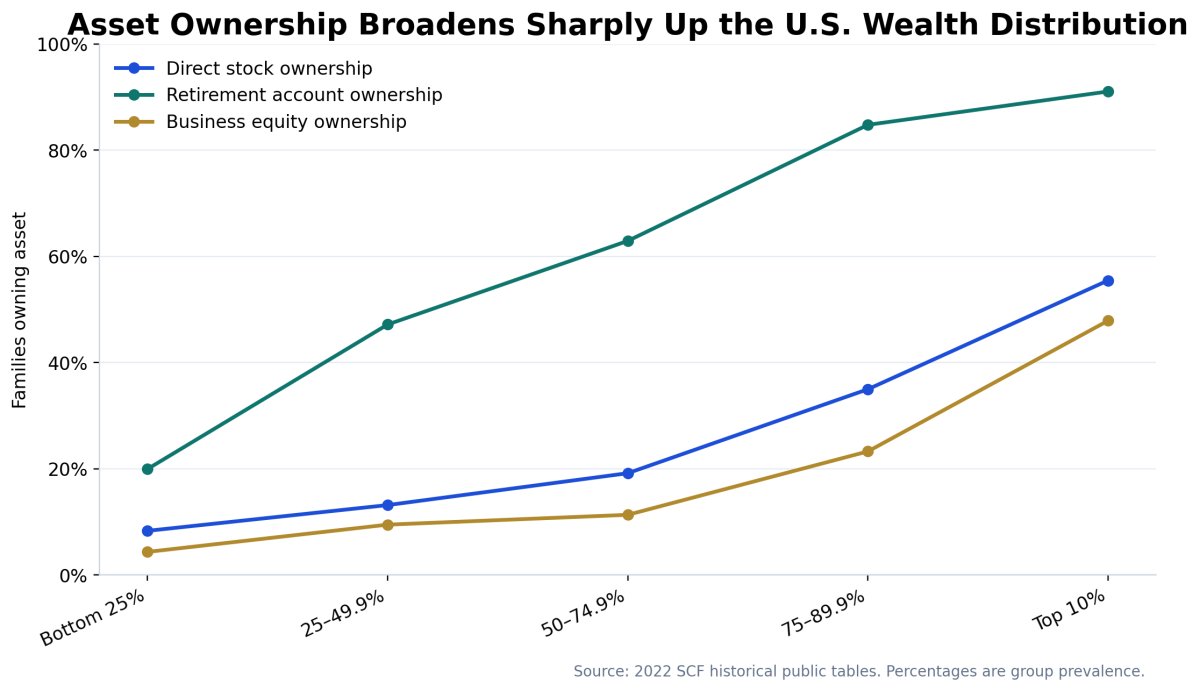
Ownership Broadens Up the Ladder
Direct stock ownership rises from about 8.3% in the bottom quarter to 55.5% in the top 10%. Retirement-account ownership rises from about 20.0% to 91.1%. Business-equity ownership rises from about 4.4% to 47.9%.
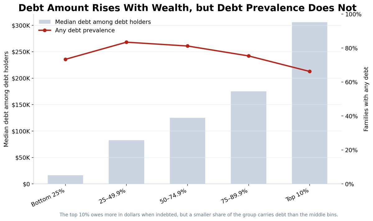
Debt Dollars Rise, Debt Prevalence Does Not
Median debt among debt-holding families rises from $16,500 in the bottom quarter to $306,000 in the top 10%. The log–log elasticity is approximately 0.411 with R² 0.991.
But the percentage of families with any debt is not monotonic. It peaks in the middle groups and falls to 66.2% in the top 10%. The regression of debt prevalence on log net worth has R² only 0.089 and p-value 0.626.
Liquidity and Capital Access
A person cannot deploy their full net worth every morning. A homeowner with $400,000 of equity may have only $8,000 in cash. A founder may be worth $20 million on a private valuation and still struggle to meet payroll without a financing round. A billionaire can borrow against concentrated stock while avoiding a taxable sale, but a market decline can trigger collateral calls.
A Practical Liquidity Stack
- Tier 1 — Immediate liquidity: cash, transaction accounts, money-market funds, immediately saleable securities.
- Tier 2 — Market liquidity: diversified listed securities, bonds, liquid funds, vested public equity.
- Tier 3 — Collateral liquidity: home equity, commercial property, equipment, receivables, business assets.
- Tier 4 — Negotiated liquidity: private company equity, partnership interests, intellectual property, future contracted income.
- Tier 5 — Trapped or costly wealth: illiquid assets with high taxes, legal restrictions, weak price discovery, or high transaction costs.
Global Financial Access
The Global Findex 2025 reports that 79% of adults globally now have an account, while only 56% say they could reliably access extra money in an emergency. This difference is crucial. Having an account is financial inclusion. Having a dependable source of emergency funds is capital resilience.
Approximately 44% of adults therefore lack reliable emergency-money access even though many may have some formal financial connection. That gap is the global shadow underneath every neat wealth percentile chart.
A person may rank above someone else in measured net worth and still face worse short-term survival constraints because their assets cannot be converted, pledged, or accessed at a reasonable cost.
The Capital Access Model
A defensible capital-access model cannot be one universal multiplier applied to net worth. Lenders do not lend against abstract wealth. They lend against cash flow, collateral, legal enforceability, volatility, loan-to-value rules, debt-service coverage, credit history, business performance, and market conditions.
The conceptual model is:
Accessible capital = f(
    liquid assets,
    lendable collateral,
    verified income and cash flow,
    debt-service capacity,
    credit quality,
    business ownership,
    asset volatility,
    legal jurisdiction,
    loan maturity,
    financing cost
)
Two-Stage Empirical Design
The correct research design is a hurdle model:
- Stage one: estimate the probability that a person can obtain meaningful formal capital.
- Stage two: conditional on access, estimate the amount and cost of capital available.
A global version would require harmonized household microdata linking wealth, income, collateral, credit use, interest rates, and denied applications. That dataset does not currently exist at the required worldwide scale. The article therefore refuses to produce fake precision.
Capital Access Score
For practical use, a person can score each component from zero to five:
| Component | Low score | High score |
|---|---|---|
| Liquidity | No emergency reserves | Large diversified liquid reserve |
| Collateral | Unsecured or depreciating assets | Low-volatility lendable assets |
| Cash flow | Unstable or unverifiable | Stable, diversified, documented |
| Debt service | High fixed obligations | Large free cash flow buffer |
| Credit structure | Short-term, variable, unsecured | Long-term, fixed, covenant-light |
| Opportunity quality | Consumption or speculative loss | Cash-producing asset with margin of safety |
The score is not a credit decision. It is a way to separate apparent wealth from real capital mobility.
Leverage: Productive, Neutral, and Destructive
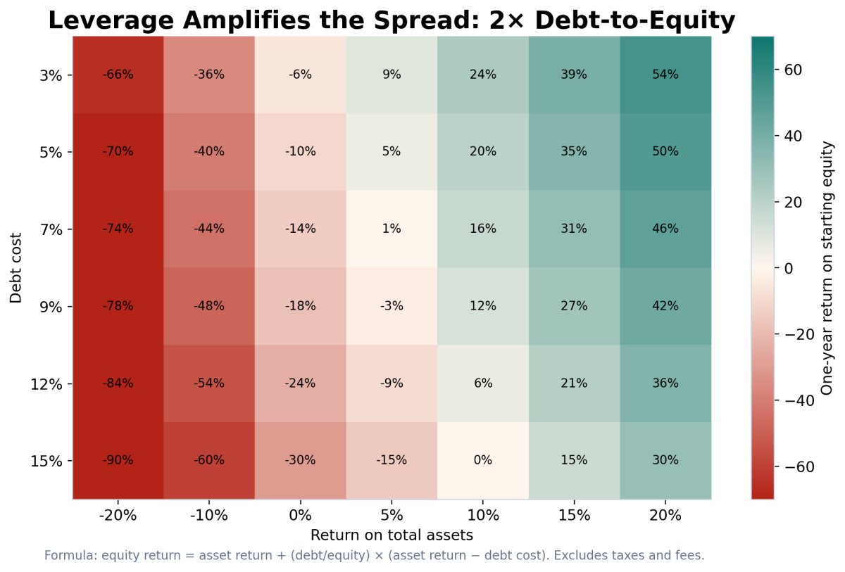
The user’s premise is correct with one critical condition: access to capital increases the ability to grow only when capital is deployed productively. Debt is a force multiplier on the spread.
Return on starting equity
= asset return
+ (debt / equity) × (asset return − debt cost)
− fees and taxes as a share of equity
Productive Leverage
Suppose $100,000 of equity supports $200,000 of debt, producing $300,000 of gross assets. If the asset earns 12% and the debt costs 7%, gross asset gains are $36,000 and interest is $14,000. Before fees and taxes, the owner creates $22,000, or 22% on starting equity.
Neutral Leverage
If the asset return equals the full financing cost, leverage increases the gross balance sheet but creates no spread. The person controls more capital without increasing equity through the leverage itself.
Destructive Leverage
If the $300,000 asset base loses 10% while the $200,000 liability still accrues 7%, the asset loses $30,000 and debt cost adds $14,000. Starting equity falls from $100,000 to approximately $56,000 before additional fees. A 10% asset loss becomes a 44% equity loss.
The Capital-Control Percentile Is Not a Wealth Percentile
A person with $100,000 in net worth and $400,000 of debt may control $500,000 of assets. That gross asset base resembles the scale controlled by someone with $500,000 in debt-free assets, but their net worth, solvency, cash-flow requirements, and drawdown risk are not the same.
The article therefore reports “capital controlled” rather than reclassifying borrowed money as wealth. This preserves the original idea—capital access expands the opportunity set—without corrupting the balance sheet.
Daily Net Worth and Daily Capital Output
“Daily net worth” is not a standard economic variable. Net worth is a stock measured at a point in time. Dividing it by 365 does not convert it into income. But the calculation is useful as a scale translator.
Daily wealth-stock equivalent = net worth / 365
At $100, the stock equivalent is $0.27 per day. At $100,000, it is about $274 per day. At $1 million, $2,740 per day. At $1 billion, $2.74 million per day. At $1 trillion, $2.74 billion per day.
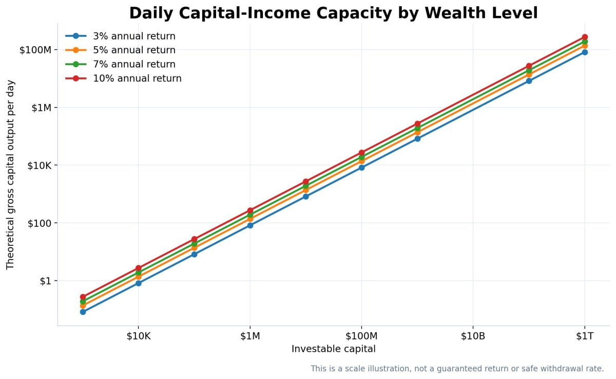
The more economically meaningful measure is theoretical capital output:
Daily gross capital output = investable capital × annual return / 365
At a 5% gross annual return, $1 million generates about $137 per day, $10 million about $1,370 per day, $1 billion about $137,000 per day, and $1 trillion about $137 million per day.
The Labor-to-Capital Transition
The ladder shows when capital income begins to rival labor income. At 5%, $100,000 produces only $5,000 annually before tax. At $1 million, it produces $50,000. At $10 million, $500,000. The economic transition occurs when capital output can fund living costs while preserving or growing the principal.
But that transition depends on asset mix. A million-dollar primary residence does not produce the same cash flow as a million-dollar diversified portfolio. A private company may produce more cash but carry far more concentration and operational risk. A pension may provide income but cannot necessarily be pledged or transferred.
Housing, Race, Age, and Structural Position
Wealth does not accumulate in a vacuum. It reflects age, homeownership, business ownership, inheritance, geography, education, income history, discrimination, family structure, market timing, and exposure to asset inflation.
Housing Status
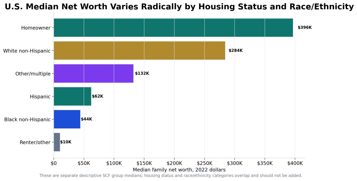
In the 2022 SCF, median net worth was approximately $396,500 for homeowners and $10,410 for renters or others. Homeownership is both an asset and a leveraged savings mechanism, but the gap also reflects selection: higher-income and higher-wealth families are more likely to become owners in the first place.
Race and Ethnicity
Published SCF medians were approximately $284,310 for White non-Hispanic families, $44,100 for Black non-Hispanic families, $62,120 for Hispanic families, and $132,200 for the other-or-multiple-race group in the historical table classification.
Age
Median family net worth rises from about $39,040 for families headed by someone under 35 to $135,300 at ages 35–44, $246,700 at 45–54, $364,270 at 55–64, and $410,000 at 65–74 before falling to approximately $334,700 for age 75 and older.
This means a raw percentile is not the only relevant benchmark. A 30-year-old with $100,000 is in a very different lifecycle position from a 70-year-old with the same amount. The national distribution answers “where are you now?” The age-conditioned distribution answers “where are you relative to your accumulation window?”
The Billionaire and Trillion-Dollar Tail
The extreme tail behaves differently from ordinary household wealth because fortunes are concentrated in controlling equity stakes, private-company valuations, public stock, intellectual property, and ownership structures that cannot be liquidated at quoted prices without changing those prices.
The 2026 Forbes annual list reported a record 3,428 billionaires globally with combined wealth of roughly $20.1 trillion. The WIR threshold model independently places the $1 billion level near the global top one-in-a-million, or approximately 5,600 adults above that threshold in its broader wealth-estimation framework. Those counts differ because the sources use different methodologies, dates, coverage, and valuation systems.
The $1 Trillion Boundary
Elon Musk crossed the $1 trillion mark on June 12, 2026 after the SpaceX public offering and later fell back below it as market prices moved. The event matters analytically because it turns $1 trillion from a hypothetical line into an observed mark-to-market boundary.
It does not mean one person possessed $1 trillion in cash. Most of the fortune consisted of equity whose quoted value depended on market prices and control stakes. Selling a large portion could create taxes, price impact, governance changes, and collateral consequences.
The $1 trillion tier is therefore the purest demonstration of the article’s central distinction:
- Mark-to-market net worth can be enormous.
- Liquid cash can be a small fraction of that amount.
- Borrowing power can still be enormous because lenders value collateral and control.
- Accessible capital may be large without being remotely equal to the headline fortune.
Why the Top Tail Moves So Fast
A founder who owns 20% of a company gains $20 billion when the company’s market value rises $100 billion. No cash must change hands in the founder’s account. The wealth change is a repricing of ownership. This is how extreme fortunes can gain or lose tens of billions in one day.
That volatility is real even though it is not cash. It changes collateral capacity, acquisition power, political influence, strategic flexibility, and the ability to finance new ventures.
Regression Results and What They Prove
| Model | Main coefficient | R² | p-value | Interpretation |
|---|---|---|---|---|
| U.S. median wealth, log trend 1989–2022 | 3.29% annual | 0.758 | 0.0002 | Typical family wealth trend |
| U.S. mean wealth, log trend 1989–2022 | 5.21% annual | 0.949 | 0.0000 | Average balance sheet trend |
| Financial assets vs. net worth, log–log | Elasticity 1.026 | 0.977 | 0.0015 | Financial assets scale almost one-for-one |
| Transaction balances vs. net worth, log–log | Elasticity 0.693 | 0.961 | 0.0033 | Cash-like balances scale sublinearly |
| Debt amount vs. net worth, log–log | Elasticity 0.411 | 0.991 | 0.0004 | Debt dollars rise, but slower than wealth |
| Any-debt prevalence vs. log net worth | -0.759 pp/log unit | 0.089 | 0.6259 | No meaningful monotonic relationship |
| Global threshold tail, Pareto-linear | Slope 0.729 | 0.992 | 0.0000 | LOOCV log-RMSE 0.541 |
| Global threshold tail, quadratic | Curvature -0.0092 | 0.996 | 0.0511 | LOOCV log-RMSE 0.504 |
What Is Strongly Supported
- The U.S. mean wealth series has grown materially faster than the median series over the SCF history.
- Financial assets rise almost proportionally with net worth across the published wealth groups.
- Transaction balances rise with wealth but more slowly than total wealth.
- Debt amounts among debtors rise with wealth, while debt prevalence itself does not show a meaningful monotonic relationship.
- The global threshold ladder is well approximated by a Pareto-style relationship, but a curved specification performs slightly better.
What Is Not Proven
- The regressions do not prove that financial assets cause wealth. Wealth allows asset acquisition, asset returns create wealth, and both directions operate.
- Five wealth-group observations do not support aggressive causal inference, even when R² is high.
- The global tail fit does not prove that one power law governs every country, year, or fortune.
- The capital-access framework does not predict an individual credit limit without person-level underwriting data.
The regressions prove scale relationships and historical divergence. They do not erase institutional context, selection, survivorship, or feedback loops.
Uncertainty, Limitations, and What Not to Claim
Global PPP Versus Market Dollars
The WIR global thresholds are designed for purchasing-power comparison. UBS and Forbes generally use market-dollar valuations. A household can move between global rankings when exchange rates change even if its domestic purchasing power does not.
Adults Versus Families
The global distribution is per adult. The U.S. SCF is per family. A married household with shared assets is not two independent adult balance sheets. This is why the article presents two separate percentile columns rather than pretending they can be merged.
Grouped Anchors Versus Microdata
The U.S. percentile curve uses official group medians and historical tables. Exact percentile estimation would require full SCF microdata with survey weights, replicate weights, and multiple-imputation combination rules. The Fed explicitly warns that ignoring those features produces incorrect standard errors.
Extreme-Tail Measurement
Academic research finds non-trivial uncertainty in top 0.1% and top 0.01% wealth estimates across both survey and tax-based methods. Forbes rankings introduce another measurement system based on public holdings, private-company estimates, known debt, and a snapshot date.
Borrowing Is Conditional
Capital access can disappear. Lenders change loan-to-value ratios, collateral haircuts, covenants, maturities, and rates. A credit line available during calm markets may be cut during the exact drawdown when it is needed.
Returns Are Not Guaranteed
The daily capital-output chart is a mathematical scale demonstration. It is not a promise that a given person can earn 3%, 5%, 7%, or 10% without volatility, tax, inflation, fees, or principal risk.
The Final Pattern Nexus Read
The global wealth system is not difficult to understand because the math is impossible. It is difficult because people keep measuring different things as though they are the same thing.
Net worth is ownership.
Liquidity is deployability.
Credit is reach.
Leverage is amplification.
Return spread is the engine.
Risk is the mechanism that can reverse the entire process.
A person with $10,000 sits around the 36.8th global percentile in this model but only near the 15.6th percentile among American families. At $100,000, the same person moves above roughly three-quarters of global adults but remains below the American median. At $1 million, the person is globally elite but still outside the American top 10%. At $10 million, the person enters the top few percent in America and the top six-hundredths of one percent globally.
Then the ladder bends vertically.
At $100 million, normal percentile language starts to fail.
At $1 billion, the relevant unit becomes one-in-a-million.
At $100 billion, it becomes a small room.
At $1 trillion, it becomes a single moving mark on a screen—an ownership claim whose value can cross the line and fall back below it in days.
But the distribution is not only a scoreboard. It is a machine.
The top owns more financial assets, more business equity, more collateral, and more access to financing. Those assets appreciate. Appreciation expands collateral. Expanded collateral allows more capital control. More capital control captures more appreciation. That is a feedback loop.
The lower distribution faces the opposite loop. Limited liquidity makes shocks expensive. Expensive credit converts emergencies into liabilities. Liabilities absorb cash flow. Reduced cash flow prevents asset acquisition. Missing the asset cycle preserves the original gap.
This does not mean mobility is impossible. It means mobility is not created by pretending debt is wealth. It is created by turning earned income, owned assets, and properly structured outside capital into a larger productive balance sheet without allowing the liability structure to outrun the cash flow.
Primary Data and Method Sources
- World Inequality Report 2026 — Global Economic Inequality
- World Inequality Report 2026 — Executive Summary
- Federal Reserve — 2022 Survey of Consumer Finances
- Federal Reserve — Distributional Financial Accounts
- World Bank — Global Findex Database 2025
- UBS — Global Wealth Report 2026
- Marta Boczon — Quantifying Uncertainties in Estimates of Income and Wealth Inequality
- Forbes — World’s Billionaires 2026 and real-time rankings
- The Guardian — Musk’s June 2026 trillion-dollar threshold and subsequent mark-to-market decline
- U.S. Census Bureau — 2024 ACS Occupancy Status
Downloadable Research Package
The accompanying package includes the full threshold ladder, regression diagnostics, assumptions, leverage scenario formulas, source log, 17 publication graphics, and the underlying CSV and JSON outputs used to build this article.
Frequently Asked Questions
What's Your Reaction?
 Like
0
Like
0
 Dislike
0
Dislike
0
 Love
0
Love
0
 Funny
0
Funny
0
 Wow
0
Wow
0
 Sad
0
Sad
0
 Angry
0
Angry
0

Founder of Pattern Nexus. I research markets, macro, geopolitics, AI, history, ancient systems, and the patterns most people overlook. I’m also building Market Radar, a trading scanner designed to read pressure, risk, confirmation, and setup quality before chasing a move. Pattern Nexus is where I connect the dots between data, history, technology, and the bigger system playing out around us.






Comments (0)