
GDP Slowed to 1.5%—But the U.S. Economy Did Not Weaken the Way the Headline Implies
Real GDP slowed to a 1.5% annual rate in Q2 2026, but the private domestic economy accelerated to 3.9% while nominal GDP grew 7.9%. This Pattern Nexus analysis separates the headline from the internal economy and explains what consumer spending, business investment, capital-goods imports, inflation, government accounting, Federal Reserve policy, and the 10-year Treasury signal actually mean.
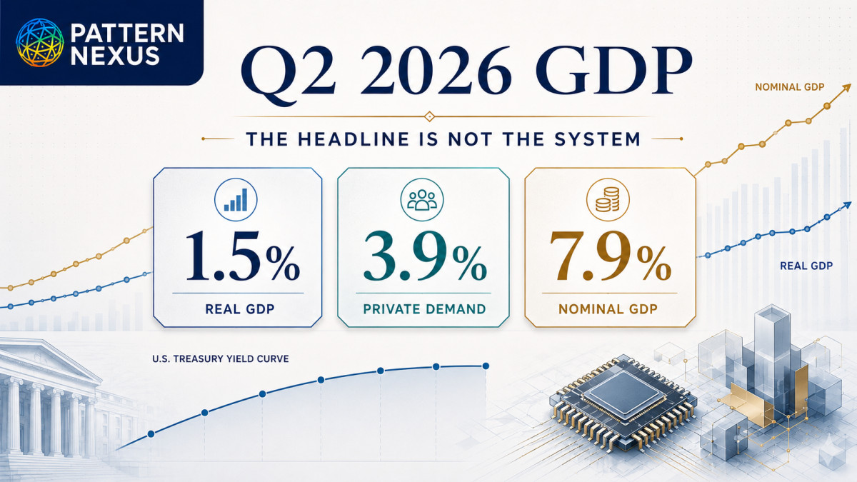
The 1.5% headline describes the total. It does not describe the system underneath it.
- Real GDP increased at a 1.5% seasonally adjusted annual rate in Q2 2026, down from 2.1% in Q1. The actual quarter-to-quarter increase was about 0.4%. This was slower growth, not contraction.[1]
- Private domestic final sales accelerated from 1.7% to 3.9%. Household spending and fixed private investment—the internal private engine—were materially stronger than the headline.[1]
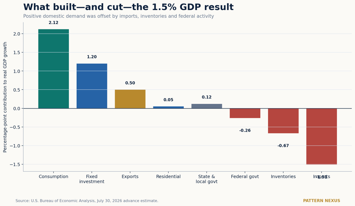
- Consumption added 2.12 percentage points to real growth. Fixed investment added another 1.20 points. Those two categories alone contributed 3.32 points before trade, inventories and government pulled the total back toward 1.5%.[2]
- Imports subtracted 1.51 points and inventories subtracted 0.67. Imports grew 11.5%, led by capital goods including telecommunications equipment, semiconductors and industrial equipment. Part of the GDP subtraction was productive capacity entering the country.[2]
- The investment cycle remained strong but concentrated. Equipment grew 15.2%, intellectual-property investment 8.8% and total nonresidential investment 8.4%. Structures fell 5.0%. This is a machinery, software, research and compute cycle—not a broad construction boom.[2]
- Nominal GDP grew 7.9% while real GDP grew 1.5%. The GDP price index rose 6.2%, gross domestic purchase prices rose 5.7%, and headline PCE rose 5.1%. Core PCE slowed to 3.4%, but the broader price system accelerated.[2]
- Real disposable personal income fell 1.5%. Aggregate spending was strong while household purchasing-power growth moved backward. That is the clearest distribution warning in the release.[2]
- Government spending fell 0.8%, led by a 12.9% drop in federal nondefense activity. Strategic Petroleum Reserve sales distorted that line: BEA says the transferred oil appeared in other components and had no direct net effect on GDP.[1]
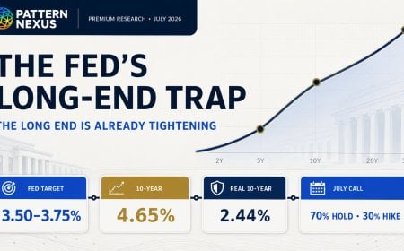
- The Fed is trapped between the internals and the financing system. Demand is too firm for an emergency cut, inflation is too high for victory, and the 10-year Treasury is already imposing restraint on housing, refinancing, commercial property and long-duration investment.
- Pattern Nexus conclusion: Q2 was not a recession quarter. It was a divided expansion—strong private demand and capital formation, weak household income conversion, broad price pressure, and a long-end constraint that makes additional short-rate tightening increasingly dangerous.
This report does not stop at the 1.5% headline. It reconstructs the contribution ledger, separates growth rates from contribution rates, compares nominal output with real output and disposable income, isolates the investment cycle, distinguishes productive capital imports from ordinary consumption leakage, audits the government-spending decline, and connects the result to the 10-year Treasury and liquidity architecture.
Six original charts are built directly from the Bureau of Economic Analysis July 30 historical-comparison workbook. Every chart uses the same advance-estimate vintage, so the internal comparisons are auditable. The article also includes the opposing case, revision risks, falsification conditions, a two-quarter scenario map and a monitoring dashboard.
The private economy accelerated while the headline economy slowed
The fastest way to misunderstand GDP is to treat the published growth rate as a uniform speed applied to every part of the economy.
Q2 did not contain one economy growing at 1.5%.
It contained consumer spending growing 3.2%, goods consumption growing 5.2%, equipment investment growing 15.2%, intellectual-property investment growing 8.8%, imports growing 11.5%, structures shrinking 5.0%, federal nondefense activity shrinking 12.9%, and real disposable personal income shrinking 1.5%.[2]
The 1.5% total is where those forces reconciled after national-accounting rules assigned each flow to consumption, investment, government, exports, imports and inventories.
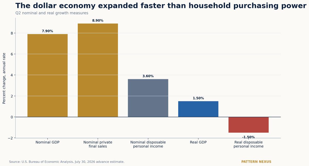
The central contradiction is not weak demand. Real final sales to private domestic purchasers accelerated to 3.9%. The contradiction is that nominal private final sales grew 8.9%, yet real disposable personal income fell 1.5%. The corporate, market and aggregate-demand layers continued expanding faster than the purchasing-power layer reaching households.
GDP is a production ledger, not a national well-being score
Gross domestic product measures the market value of final goods and services produced inside the United States. The expenditure identity is commonly written:
Each term answers an accounting question. None of them, by itself, answers whether the median household became more secure, whether the capital stock became more productive, whether growth was debt-financed, or whether the economy increased its strategic independence.
Real GDP
Output after BEA removes estimated price changes. It is the standard headline growth measure.
Nominal GDP
Output measured in current dollars. It matters for revenue, taxes, wages, profits and debt ratios.
Final sales
GDP excluding inventory accumulation. It shows whether current production reached a final buyer.
Private domestic final sales
Consumer spending plus private fixed investment. It removes trade, government and inventories.
GDI
The income-side measure of the same production. It is unavailable in the Q2 advance release and arrives later.
Disposable income
Income available to households after taxes and transfers. Real disposable income is closer to purchasing-power experience.
The annualized convention also matters. BEA reports the rate that would prevail if one quarter's pace continued for a full year. Q2 real GDP rose about 0.4% from Q1; annualizing that movement produces 1.5%. Annualization improves comparison but magnifies temporary movements.
The headline decelerated; the private engine and dollar economy accelerated
| Measure | Q1 2026 | Q2 2026 | Change in signal |
|---|---|---|---|
| Real GDP | 2.1% | 1.5% | Slower aggregate real growth |
| Real final sales of domestic product | 1.9% | 2.2% | Final demand for domestic output improved |
| Real final sales to domestic purchasers | 2.2% | 3.1% | Domestic final demand strengthened |
| Real final sales to private domestic purchasers | 1.7% | 3.9% | Private internal engine accelerated sharply |
| Current-dollar GDP | 5.8% | 7.9% | Nominal scale accelerated |
| Nominal private domestic final sales | 5.9% | 8.9% | Private dollar spending accelerated |
| Real disposable personal income | 0.9% | −1.5% | Household purchasing power contracted |
| Gross domestic purchases prices | 3.6% | 5.7% | Broad domestic price pressure accelerated |
| Core PCE prices | 4.4% | 3.4% | Underlying consumer inflation cooled |
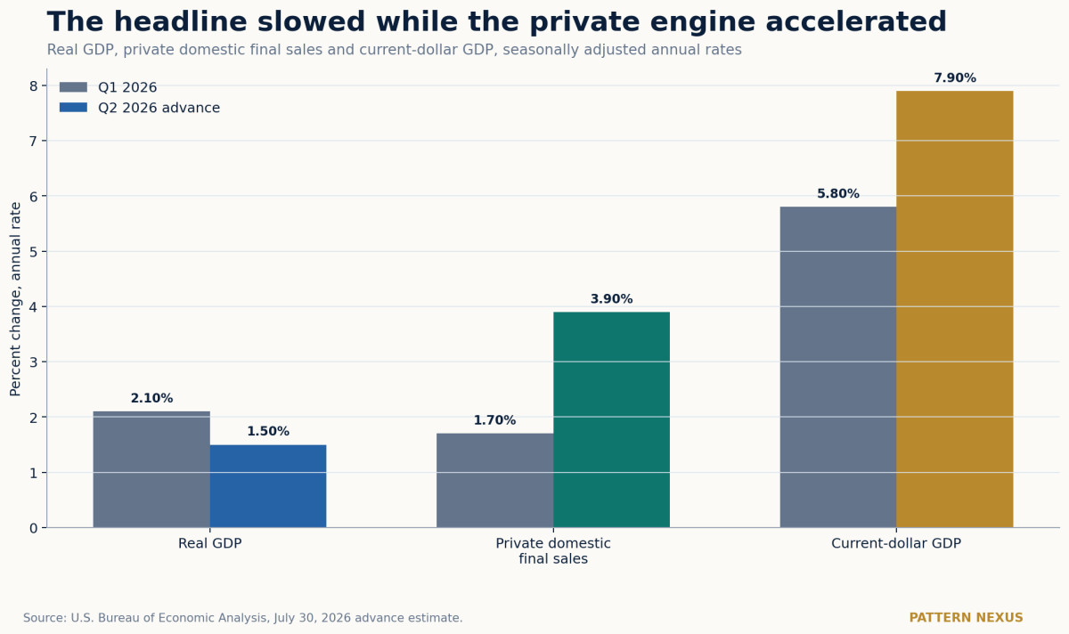
The most important spread is 2.4 percentage points: private domestic final sales grew 3.9% while real GDP grew 1.5%. Trade, inventories and government explain the gap.
The second spread is 6.4 points: nominal GDP grew 7.9% while real GDP grew 1.5%. Prices explain most of that gap.
The third spread is 5.4 points: nominal private final sales grew 8.9% while real disposable income fell 1.5%. That is the distribution and purchasing-power gap.
Consumption and fixed investment built a 3.32-point domestic expansion
A component's growth rate and its contribution to GDP are different numbers. Equipment can grow 15.2% but contribute less than consumption because equipment is a smaller share of the economy. Contribution analysis weights each category by its economic size.
| Component | Contribution | What it means |
|---|---|---|
| Personal consumption | +2.12 points | The household sector supplied more than the final 1.5% headline by itself. |
| Fixed investment | +1.20 | Productive capital formation was the second major engine. |
| Exports | +0.50 | Petroleum-related goods led export growth. |
| Residential investment | +0.05 | Housing investment was positive but weak. |
| State and local government | +0.12 | Local public activity remained slightly positive. |
| Federal government | −0.26 | Nondefense activity and SPR accounting pulled the public component lower. |
| Private inventories | −0.67 | Businesses accumulated inventory more slowly or drew stock relative to Q1. |
| Imports | −1.51 | Foreign production met part of U.S. demand and was removed from domestic output. |
The ledger resolves the apparent contradiction. Domestic demand was capable of producing a much stronger headline. The GDP identity removed production created abroad, removed the inventory slowdown, and incorporated the federal decline.
The consumer did not disappear, but spending is not the same as comfort
Real consumer spending grew 3.2%. Goods rose 5.2%, durable goods 6.8%, nondurable goods 4.4%, and services 2.2%. BEA identified prescription drugs, new light trucks, furniture, food services and accommodations, financial services and nonprofit activity as leading contributors.[1]
This breadth argues against a Q2 demand collapse. Both goods and services expanded. Durable-goods growth also suggests households and businesses were still willing or able to make larger purchases.
But GDP records spending regardless of how comfortable that spending feels. A household paying more for medicine, insurance, lodging, food services or transportation increases nominal activity. The same household may have less discretionary cash after the transaction.
Three financing channels can keep consumption strong while household conditions weaken:
- Income concentration: high-income and asset-owning households can support aggregate spending even if the median household slows.
- Credit substitution: revolving balances, installment loans and delayed repayment can bridge a temporary income gap.
- Essential-price substitution: households spend more on required goods and services while cutting less visible discretionary categories.
The release does not prove which channel dominated. The decline in real disposable personal income makes it dangerous to interpret aggregate consumption as proof of broad household strength.
The United States generated more dollars than real output
Current-dollar GDP rose 7.9%. Real GDP rose 1.5%. The GDP implicit price deflator increased 6.3%, almost exactly describing the conversion loss between the two layers.[2]
This does not mean nominal growth is fake. Nominal dollars pay wages, service debt, support profits, determine tax receipts and set collateral values. The problem is that nominal growth can preserve financial ratios while living standards stagnate.
Corporate layer
Nominal sales can rise with prices even when real unit growth is limited.
Fiscal layer
Nominal income and spending can raise tax receipts and temporarily improve debt ratios.
Household layer
Real disposable income determines whether nominal gains increase purchasing power.
Asset layer
Nominal liquidity and cash flow can support asset prices despite weak affordability.
This is the same architecture behind the Pattern Nexus “52-cent economy” work. GDP, employee compensation, wages, after-tax income and after-essential-cost retention are nested layers. A positive aggregate total does not guarantee an equal lived outcome.
Real disposable personal income fell 1.5%
This is the number most likely to be lost beneath the GDP headline.
Nominal disposable personal income rose 3.6%, slower than nominal GDP and slower than the broad price measures. After price adjustment, real disposable income fell 1.5%.[2]
The household sector therefore entered Q3 with strong aggregate spending but weaker income conversion. That combination can persist for a time. It cannot persist indefinitely without some adjustment through savings, debt, lower consumption, higher wages, lower inflation or transfers.
This is also why a recession cannot be diagnosed from GDP alone. Household income can deteriorate before aggregate output contracts. Alternatively, productivity and wage gains can restore income before spending breaks. The direction of that reconciliation is one of the most important Q3 and Q4 questions.
Equipment grew 15.2%; structures fell 5.0%
Gross private domestic investment grew 3.0%, but the aggregate hides a major internal split. Fixed investment grew 7.0%. Nonresidential investment grew 8.4%. Equipment surged 15.2%, intellectual-property products grew 8.8%, residential investment rose only 1.5%, and structures contracted 5.0%.[2]
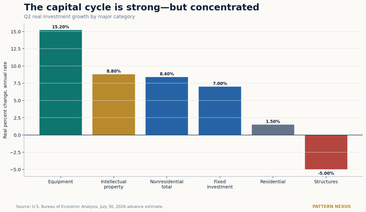
This composition matters more than the total.
- Equipment expands physical productive capacity and may include information-processing, industrial and transportation systems.
- Intellectual property includes software and research and development—the core intangible infrastructure of AI and automation.
- Structures are exposed to long-duration financing, construction costs, permits and the higher 10-year Treasury transmission.
- Residential investment remains constrained by mortgage rates and affordability even when national output is positive.
The economy is choosing assets with faster deployment and clearer strategic returns while hesitating on long-lived structures. That is rational under high rates and rapid technological change. It also concentrates growth in firms capable of financing compute, equipment, software and research.
The productivity upside is real. If the 15.2% equipment surge translates into output per hour, the United States can grow real capacity without matching inflation. If it remains a narrow spending wave around imported hardware and concentrated platforms, nominal investment may outrun broad productivity gains.
Imports removed 1.51 points—but capital imports are not ordinary weakness
Exports grew 4.5% and contributed 0.50 point to GDP. Goods exports grew 8.9%, led by petroleum and related products. Services exports fell 3.3%.
Imports grew 11.5% and subtracted 1.51 points. Goods imports rose 14.7%, while services imports were nearly flat. BEA says the goods increase was led by capital goods excluding autos—telecommunications equipment, semiconductors and related devices, and industrial equipment.[1]
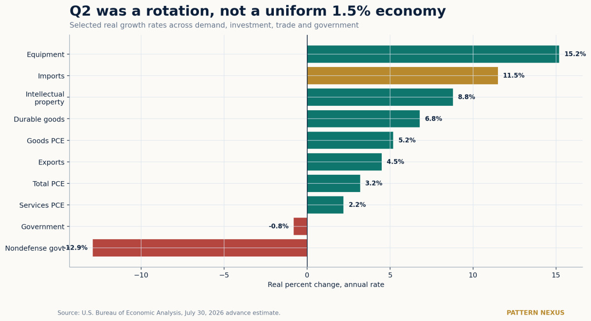
Imports are correctly subtracted because GDP measures production inside the United States. But two economically different events share the same accounting sign:
Consumption leakage
Imported final goods meet current demand while domestic productive capacity does not increase.
Productive leakage
Imported equipment reduces current GDP but expands the future domestic capital stock.
The capital-goods composition makes the Q2 trade subtraction less recessionary than the number appears. It may still reveal a strategic dependency: the United States is expanding AI, communications and industrial capacity partly through foreign production.
Inventories removed 0.67 point without proving final demand weakened
Changes in private inventories subtracted 0.67 percentage point from Q2 growth. Wholesale trade was the largest source of the decline.[1]
Inventory accounting is unintuitive. GDP depends on the change in inventory investment, not simply whether inventory levels rose or fell. Businesses can continue adding stock and still subtract from GDP if they add it more slowly than in the previous quarter.
A negative inventory contribution can carry at least three meanings:
- Demand outran supply: firms sold goods faster than they replenished them, potentially creating future restocking.
- Businesses became cautious: firms reduced orders because they expect slower sales.
- Trade and timing shifted: imported capital or goods arrived in a pattern that moved stock across quarters.
The 3.9% private final-sales reading makes a pure demand-collapse interpretation less convincing. If final demand remains firm, the inventory drag can reverse and add to a later quarter. If firms were preparing for weaker demand, the negative contribution becomes an early warning.
Federal nondefense activity fell 12.9%, but the oil transfer distorted the signal
Total government consumption and investment fell 0.8% and subtracted 0.14 point from growth. Federal activity fell 4.1%; defense rose 2.4%; nondefense fell 12.9%; and state and local activity grew 1.1%.[2]
BEA attributes the federal nondefense pattern primarily to Strategic Petroleum Reserve crude sales. In national accounting, the sale is deducted from government consumption. The oil appears as an increase elsewhere, leaving no direct net effect on GDP.[1]
This distinction matters for two reasons.
First, the government line does not represent a simple disappearance of demand. Part of it is an institutional transfer of an existing asset.
Second, the physical system still changes. Selling strategic oil can support current supply and soften near-term price pressure, but it reduces the inventory available for a future disruption. GDP can show no direct effect while national resilience declines.
Core PCE cooled while nearly every broader price measure accelerated
Headline PCE inflation rose from 4.6% to 5.1%. Core PCE slowed from 4.4% to 3.4%. That looks like underlying improvement beneath an energy- and goods-driven headline shock.
But the broader measures were less comforting. Gross domestic purchase prices accelerated from 3.6% to 5.7%. The same measure excluding food and energy accelerated from 3.3% to 4.7%. The GDP price index accelerated from 3.6% to 6.2%. The GDP implicit deflator rose 6.3%.[2]
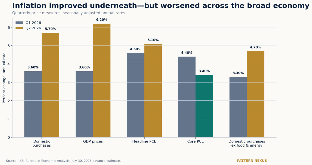
The price measures answer different questions:
- PCE measures prices paid for household consumption, including expenditures made on households' behalf.
- Gross domestic purchases prices measure goods and services purchased by U.S. residents, including imports.
- GDP prices measure prices attached to domestically produced output and exclude imports.
When domestic purchase prices and GDP prices both accelerate, the inflation problem cannot be dismissed as one imported-energy line. When core PCE simultaneously cools, the system is sending a mixed signal: household underlying inflation may be improving while broader production and purchase prices remain stressed.
This is exactly the kind of composition that traps monetary policy. A central bank can see enough disinflation to hesitate and enough broad inflation to avoid declaring victory.
The Fed controls overnight money; the 10-year prices the duration economy
On July 29, the Federal Reserve held the federal funds target at 3.50%–3.75%. Beth Hammack, Neel Kashkari and Lorie Logan preferred a 25-basis-point increase.[4]
Q2 gives the dissenters a case: private domestic demand grew 3.9%, nominal GDP grew 7.9%, domestic purchase prices rose 5.7%, and headline PCE rose 5.1%.
Q2 also gives the majority a case: real GDP slowed to 1.5%, real disposable income fell 1.5%, structures contracted, inventories weakened, and core PCE slowed.
The false debate asks whether 3.50%–3.75% is sufficiently restrictive. The better question asks what rate households, businesses and government actually refinance against.
Housing
Mortgage rates price from the long end, spreads and prepayment risk—not directly from overnight policy.
Commercial property
Capitalization rates and refinancing costs respond to Treasury duration and credit spreads.
Business investment
Long-lived structures face the duration rate even while software and equipment can be funded faster.
Federal finance
Higher term premiums roll gradually into Treasury interest expense and future issuance.
The investment split already shows the transmission. Equipment and intellectual property are expanding; structures are contracting. The system is favoring assets with faster deployment and shorter payback while punishing duration.
Another short-rate hike may slow private demand, but it cannot produce semiconductors, lower oil, rebuild the SPR or directly compress the term premium. It risks tightening the same rate-sensitive sectors already carrying the weakest internal readings.
A cut is not clean either. Cutting into 5%–6% broad price pressure could weaken the dollar, raise commodity prices or prevent long yields from falling if markets interpret the action as inflationary.
Aggregate resilience can coexist with household compression
GDP does not distribute itself evenly. The Q2 release contains several channels capable of widening the gap between aggregate strength and household experience.
- Capital concentration: equipment, software and research investment accrue first to firms with scale, credit access and strategic positioning.
- Import dependence: productive equipment enters the country, but the current production income accrues abroad.
- Inflation conversion: nominal GDP, sales and asset values rise faster than real output and real disposable income.
- Duration inequality: existing fixed-rate borrowers are protected while new buyers, refinancers and younger households face current rates.
- Spending concentration: high-income households can keep aggregate consumption strong while lower-income households reduce discretionary demand.
This is why “GDP is positive” is not a complete answer to public economic dissatisfaction. The statistic can be accurate and the dissatisfaction can also be accurate. They refer to different layers.
The countercase: Q2 may be stronger and healthier than this framework implies
A serious analysis must identify the strongest opposing interpretation.
Private demand is the correct signal
Real private domestic final sales grew 3.9%. Consumption and fixed investment added 3.32 points. Imports and inventories are volatile. On this view, the 1.5% headline understates a healthy internal economy.
Capital imports are a productivity investment
Telecommunications equipment, semiconductors and industrial equipment can raise future output. The import subtraction is a temporary accounting cost of building a more productive domestic system.
Core PCE is the policy signal
Core PCE slowed from 4.4% to 3.4%. If energy and conflict effects fade, broader inflation measures may follow, allowing real income to recover without a recession.
Inventory drag can reverse
If final demand remains firm, businesses must rebuild stock. The −0.67-point inventory contribution could become a positive contribution later.
Productivity can solve the rate problem
Equipment, software and research investment may lift productivity, profits and real wages enough to validate high long rates without breaking the economy.
This countercase becomes the base case if real disposable income rebounds, core inflation continues falling, private final demand remains above 3%, equipment investment spreads into measurable productivity, and long yields stabilize without a credit event.
The advance estimate is a map drawn before every road is visible
The July 30 release is the advance estimate. BEA used complete data for some months and categories, partial data for others, and judgmental trends or projections where June information was incomplete. Software and research estimates, some construction data, inventories and trade details are especially capable of revision.[1]
The second estimate arrives August 26 with corporate profits. The annual national, industry and regional update begins September 30.[1]
GDI is also missing from the advance release. GDP measures expenditure; GDI measures income generated by production. In theory they are equal. In real time they diverge because the source data differ. The average of GDP and GDI can provide a better read once both are available.
| Revision-sensitive area | Current conclusion | What would change the thesis |
|---|---|---|
| Private final sales | Strong at 3.9% | A material downward revision would weaken the non-recession case. |
| Equipment and IP | Strong capital cycle | Large downward revisions would weaken the productivity thesis. |
| Inventories | −0.67-point drag | A smaller drag would raise underlying GDP; a larger drag could increase restocking potential or caution. |
| Real disposable income | −1.5% | An upward revision would reduce the household-stress warning. |
| GDI and profits | Unavailable | Weak income and profits would reveal more fragility than expenditure GDP shows. |
Four paths through Q3 and Q4
| Scenario | Required conditions | GDP, inflation and rate path |
|---|---|---|
| Base: nominal resilience, real cooling | Private demand remains positive; core inflation eases slowly; real income stabilizes; long yields remain restrictive. | Real GDP stays positive but uneven. The Fed holds. Rate-sensitive sectors lag capital-intensive sectors. |
| Productivity escape | Equipment and IP spending lift output per hour; imported capital is deployed domestically; core inflation falls. | Real growth rises toward nominal growth. Real income recovers. The 10-year can fall modestly without recession. |
| Inflation trap | Energy and supply shocks persist; broad price measures remain near 5%; private demand stays firm. | The Fed remains pinned or hikes. The 10-year stays high. Housing, structures and weaker borrowers deteriorate beneath positive GDP. |
| Long-end break | Refinancing, housing, commercial property and consumer credit transmit the duration shock into jobs and spending. | Private final demand falls, inventories rise involuntarily or are liquidated, GDP weakens, and liquidity support arrives before clean inflation victory. |
The most likely near-term outcome is not a clean boom or immediate recession. It is continued division: strategic capital formation and higher-income consumption support aggregate demand while structures, affordability and household purchasing power remain under pressure.
Scenario note: These are conditional analytical paths, not statistically calibrated probabilities or individualized investment advice.
The dashboard that decides which GDP story is real
| Indicator | Bullish confirmation | Bearish confirmation |
|---|---|---|
| Private domestic final sales | Remains above 3% | Revised below 2% or falls sharply in Q3 |
| Real disposable personal income | Returns positive and outpaces consumption | Remains negative while credit and delinquencies rise |
| Equipment and IP investment | Stays strong and broadens into productivity | Falls after one concentrated import-and-spending surge |
| Structures and housing | Stabilize as long yields fall | Contraction deepens despite positive GDP |
| Core PCE | Moves toward 2% without demand collapse | Reaccelerates or remains above 3% |
| Domestic purchase prices | Converge downward toward core PCE | Remain near 5%–6% |
| Inventories | Restocking follows firm final demand | Inventory liquidation reflects collapsing orders |
| GDI and corporate profits | Confirm expenditure-side resilience | Reveal an income-side slowdown beneath GDP |
| 10-year Treasury | Falls through disinflation and lower term premium | Stays elevated as growth and real income weaken |
| Credit spreads and delinquencies | Remain contained | Broaden from weaker households into business credit |
What would invalidate the stronger Pattern Nexus warning?
- Real disposable income rebounds quickly and remains positive.
- Core and broad inflation measures converge toward 2%–3%.
- The 10-year falls without a recession or financial accident.
- Equipment and intellectual-property investment generate measurable productivity and wage growth.
- Structures and residential investment stabilize.
- GDI and corporate profits confirm the strength visible in private final sales.
If those conditions develop, Q2 should be read as a healthy capital-deepening quarter temporarily obscured by trade, inventories and energy-related price pressure.
The economy is expanding through the channels least visible in the headline
The public sees 1.5% and asks whether the economy is weak.
The contribution ledger sees consumption adding 2.12 points and fixed investment adding 1.20.
The capital ledger sees equipment growing 15.2% and intellectual property growing 8.8%.
The trade ledger sees capital goods entering the country while imports subtract 1.51 points.
The household ledger sees real disposable income falling 1.5%.
The price ledger sees nominal GDP growing 7.9%, GDP prices rising 6.2%, and real output growing only 1.5%.
The physical ledger sees strategic oil transferred out of the SPR even when GDP records no direct net effect.
The financing ledger sees structures contracting while equipment and software expand.
The monetary ledger sees three officials asking for another hike while the duration economy is already being restrained by the long end.
This does not prove a recession is imminent.
It proves the next phase depends on conversion.
Can imported equipment become domestic productive capacity?
Can software and research become measurable output per hour?
Can core disinflation pull broad prices lower?
Can nominal income reach households faster than essential costs?
Can the 10-year fall without a break large enough to force liquidity intervention?
If the answer is yes, the United States exits through productivity: more real output, higher wages, lower inflation and a manageable long end.
If the answer is no, the same data exit through fracture: weaker structures, tighter household balance sheets, slower final demand, falling employment and eventual liquidity support.
Frequently Asked Questions
Did the U.S. economy contract in Q2 2026?
No. Real GDP increased at a 1.5% annual rate, equal to approximately 0.4% from Q1 to Q2 before annualization.[1]
Why did GDP slow if private demand accelerated?
Imports, inventories and government activity pulled the total below the growth generated by consumption and fixed investment. Private domestic final sales increased 3.9%.
What contributed most to growth?
Personal consumption added 2.12 percentage points and fixed investment added 1.20. Imports subtracted 1.51 and inventories subtracted 0.67.[2]
Was business investment strong?
Yes, but concentrated. Equipment grew 15.2% and intellectual-property investment grew 8.8%, while structures fell 5.0%.
Why did imports subtract so much?
GDP measures domestic production. Imports are produced abroad and must be removed. Q2 imports included telecommunications equipment, semiconductors and industrial equipment that may support future U.S. production.
Was inflation improving or worsening?
Both signals appeared. Core PCE slowed to 3.4%, but headline PCE rose to 5.1%, domestic purchase prices to 5.7%, and GDP prices to 6.2%.
What was the clearest household warning?
Real disposable personal income fell 1.5% even as consumption and nominal GDP expanded.
Did government spending really collapse?
Federal nondefense activity fell sharply, but Strategic Petroleum Reserve sales distorted the line. BEA says the transferred oil appeared elsewhere and had no direct net GDP effect.
Does the report support a Fed hike or cut?
It supports neither cleanly. Strong private demand and broad inflation argue against a rapid cut. Slower real GDP, falling real disposable income and long-end restraint argue against another automatic hike.
Is 1.5% the final number?
No. It is the advance estimate. The second estimate is scheduled for August 26, followed by the annual national-account update beginning September 30.
Research and Data Sources
- U.S. Bureau of Economic Analysis, GDP (Advance Estimate), 2nd Quarter 2026, July 30, 2026.
- U.S. Bureau of Economic Analysis, 2026 Q2 Advance Estimate Historical Comparisons Workbook, July 30, 2026.
- U.S. Bureau of Economic Analysis, National Income and Product Accounts Interactive Tables.
- Board of Governors of the Federal Reserve System, FOMC Statement, July 29, 2026.
- Board of Governors of the Federal Reserve System, Implementation Note, July 29, 2026.
- Board of Governors of the Federal Reserve System, Monetary Policy Report, July 2026.
Chart method
Figures 1–6 are original Pattern Nexus charts created from the BEA July 30 historical-comparison workbook. Growth rates and price changes are seasonally adjusted annual rates. Contribution figures are percentage-point contributions to the annualized change in real GDP. They must not be added to component growth rates because the two measures answer different questions.
Q2 2026 values are advance estimates. Historical comparisons in the workbook use the data vintage available on July 30, 2026. Later BEA releases and the September annual update may revise the current quarter and historical series.
Editorial note: The article title image is intentionally excluded from the HTML body and belongs in the post Image field. Figures 1–6 use the final Pattern Nexus upload URLs supplied for this article.
Frequently Asked Questions
What's Your Reaction?
 Like
0
Like
0
 Dislike
0
Dislike
0
 Love
0
Love
0
 Funny
0
Funny
0
 Wow
0
Wow
0
 Sad
0
Sad
0
 Angry
0
Angry
0

Founder of Pattern Nexus. I research markets, macro, geopolitics, AI, history, ancient systems, and the patterns most people overlook. I’m also building Market Radar, a trading scanner designed to read pressure, risk, confirmation, and setup quality before chasing a move. Pattern Nexus is where I connect the dots between data, history, technology, and the bigger system playing out around us.



Comments (0)